# K-Nearest Neighbor (KNN) Classifier k - 近邻算法

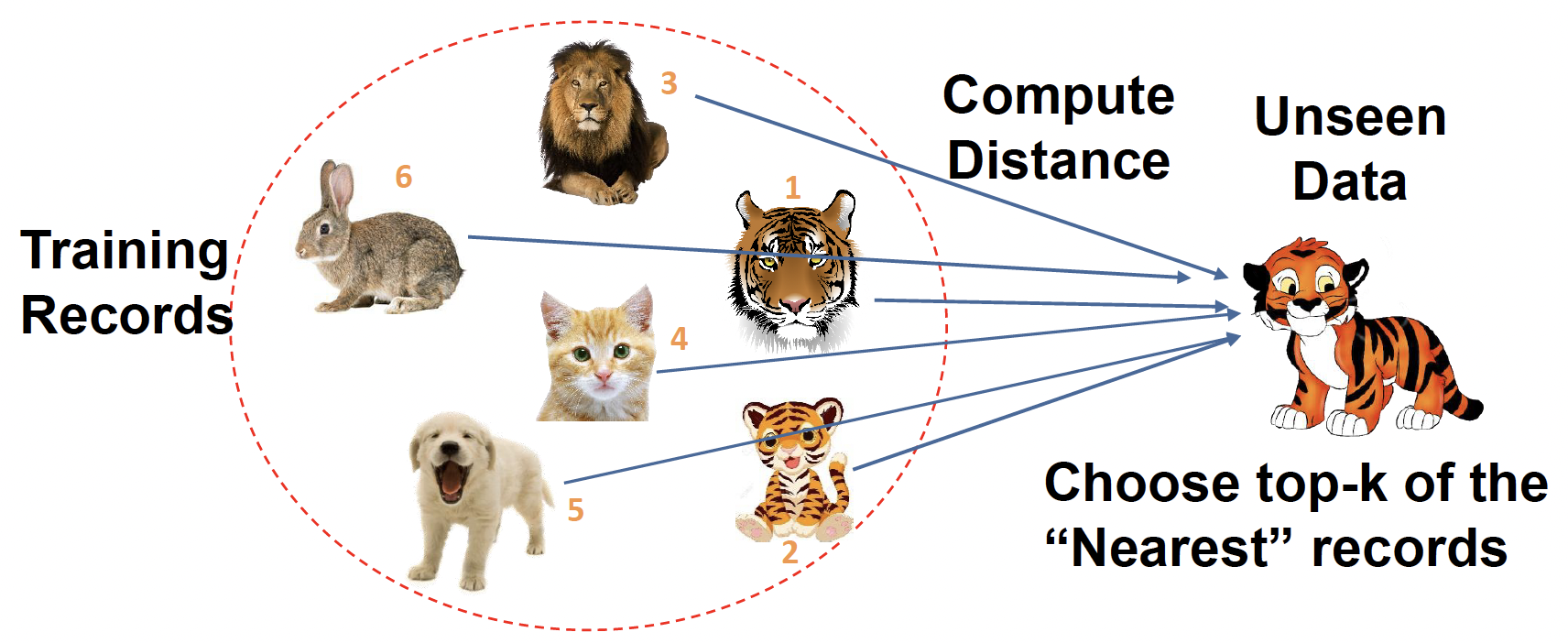
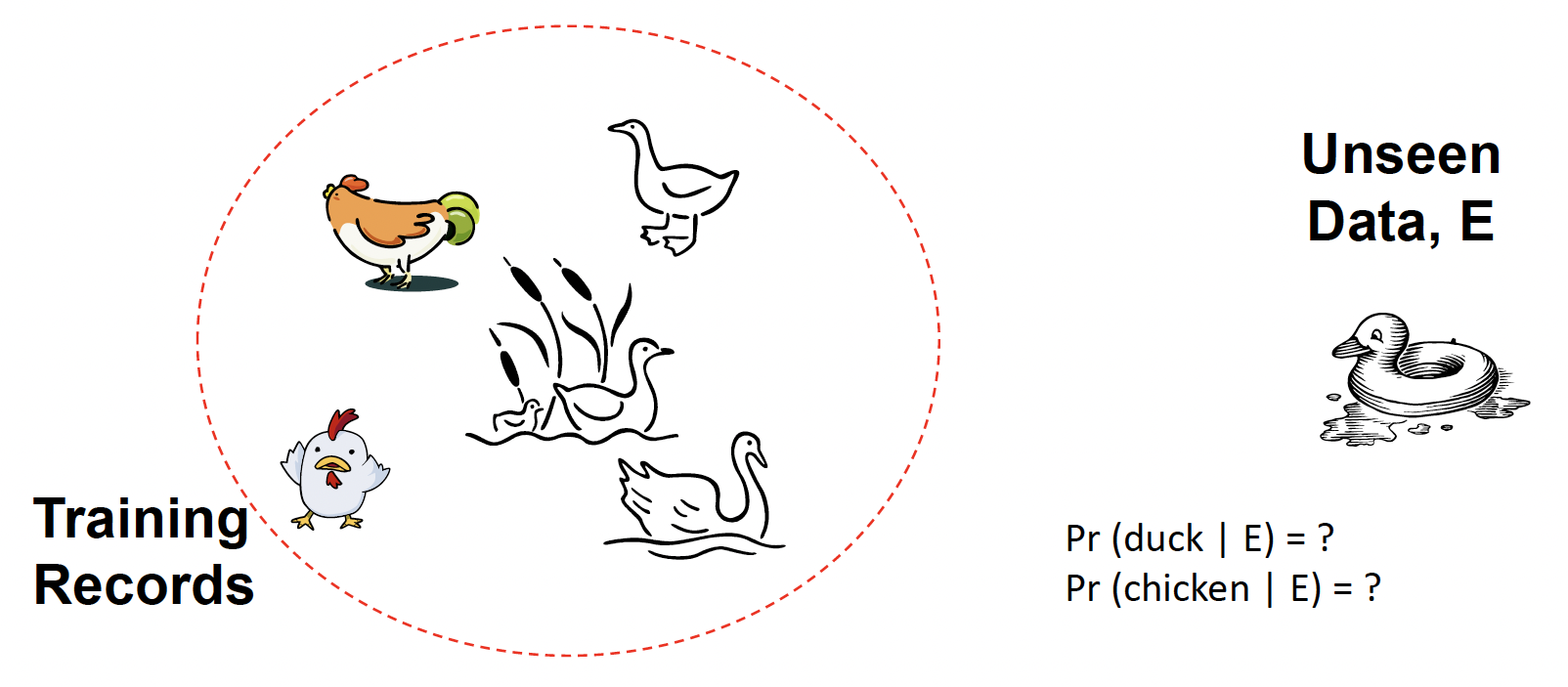
• Problem: Identify which animal the given object it is
  问题：识别给定对象是哪种动物

• Features: weights, age, gender, stripes, size, etc
  特征：体重、年龄、性别、条纹、大小等

• KNN classifier is a simple classification algorithm
  KNN 分类器是一种简单的分类算法
  The idea behind is to classify new examples based on their similarity to or distance from examples we have seen before (in training set).
  根据新示例与之前（在训练集中）看到的示例的相似性或距离对其进行分类。

# Build a KNN Classifier

1. Calculate distances between target and instances in train set
   计算目标与训练集中实例之间的距离
2. Identify the top-K nearest neighbor (choose an odd number for K!)
   确定前 K 个最近邻居 (为 K 选择一个奇数！)
3. Predict labels and validate with truth
   预测标签并用事实来验证
   • How to predict? 如何预测？
     The predicted class = the majority class label in those neighbors
     预测类 = 这些邻居中的多数类标签

K = 1，距离最近的是 1 号老虎，预测就是老虎
K = 2，前 2 个最近邻居，是 1 号 2 号老虎，预测是老虎
For example, among top 3 picks (K = 3), 2/3 are tigers!!
例如，在前 3 个选择 (K = 3) 中，2/3 是老虎！！
K = 4，前 4 个最近邻居，2/4 是老虎，预测还是老虎
K 值最好选择奇数，偶数可能无法作出判断

# Distance Measures 距离测量

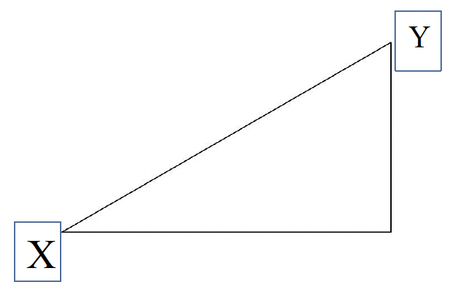
Assume there are n features, and two examples: X and Y

1. Consider two vectors 定义两个向量

   • Rows in the data matrix 代表数据矩阵中的两行

   $$X=\left\langle x_{1}, x_{2}, \cdots, x_{n}\right\rangle$$

   $$Y=\left\langle y_{1}, y_{2}, \cdots, y_{n}\right\rangle$$

   X 和 Y 分别表示两个 object，$x_{1}, x_{2}$ 等表示 X 的不同特征的值
   X 和 Y 距离越近，两者越相似

2. Common Distance Measures 常见距离度量

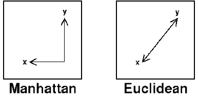
   • Manhattan distance: ( aggregation of two right angle legs )
     曼哈顿距离：两条直角坐标的聚合

   $$\operatorname{dist}(X, Y)=\left|x_{1}-y_{1}\right|+\left|x_{2}-y_{2}\right|+\cdots+\left|x_{n}-y_{n}\right|$$

   • Euclidean distance: ( length of hypotenuse )
     欧几里得距离：斜边的长度

   $$\operatorname{dist}(X, Y)=\sqrt{\left(x_{1}-y_{1}\right)^{2}+\cdots+\left(x_{n}-y_{n}\right)^{2}}$$

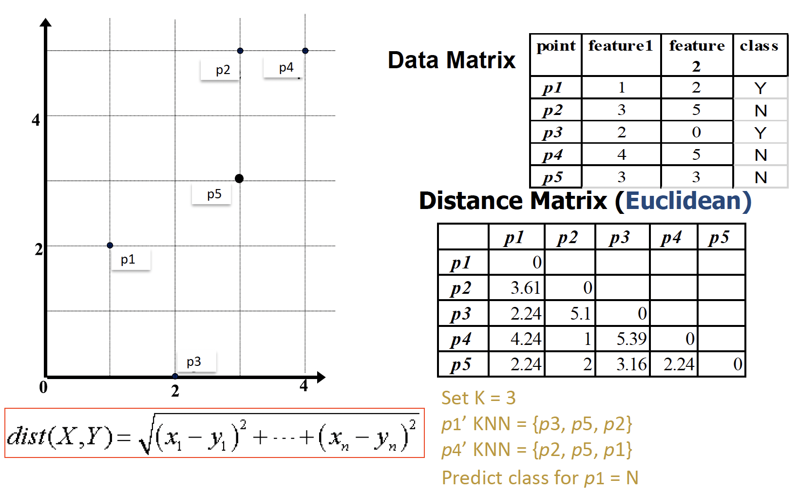
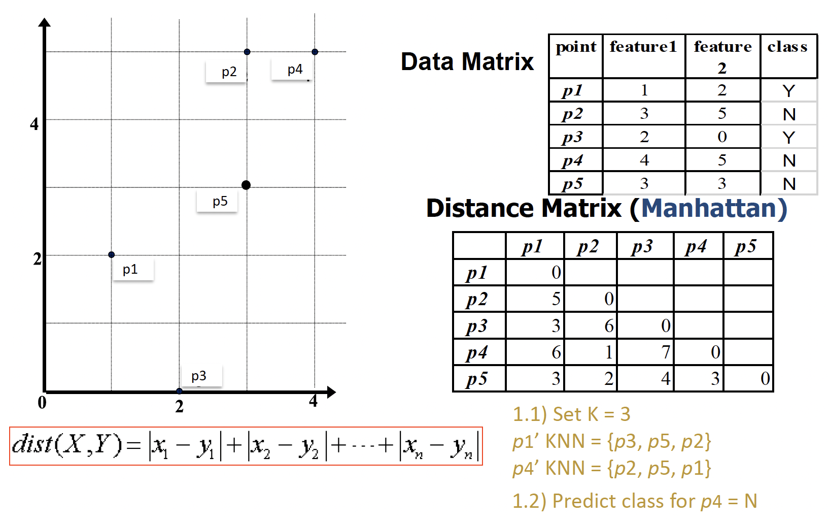
Example

用 Manhattan distance 做练习
先按公式，计算 p1 和其他四个之间的距离值
设定 K = 3，则从小到大取 3 个，分别是 p3、p5、p2
这三个的 class 分别为 Y、N、N，可见大多数都是 N，因此 p1 的预测值为 N
而实际 p1 的 class 是 Y，所以预测值是错误的

# General Questions for Classifications

• What are the required data types by an algorithm
  算法所需的数据类型是什么
• Is there an overfitting problem?
  是否存在过拟合问题
• Is there a training learning process?
  是否有训练学习过程？

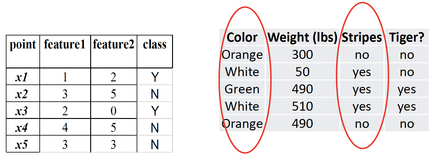
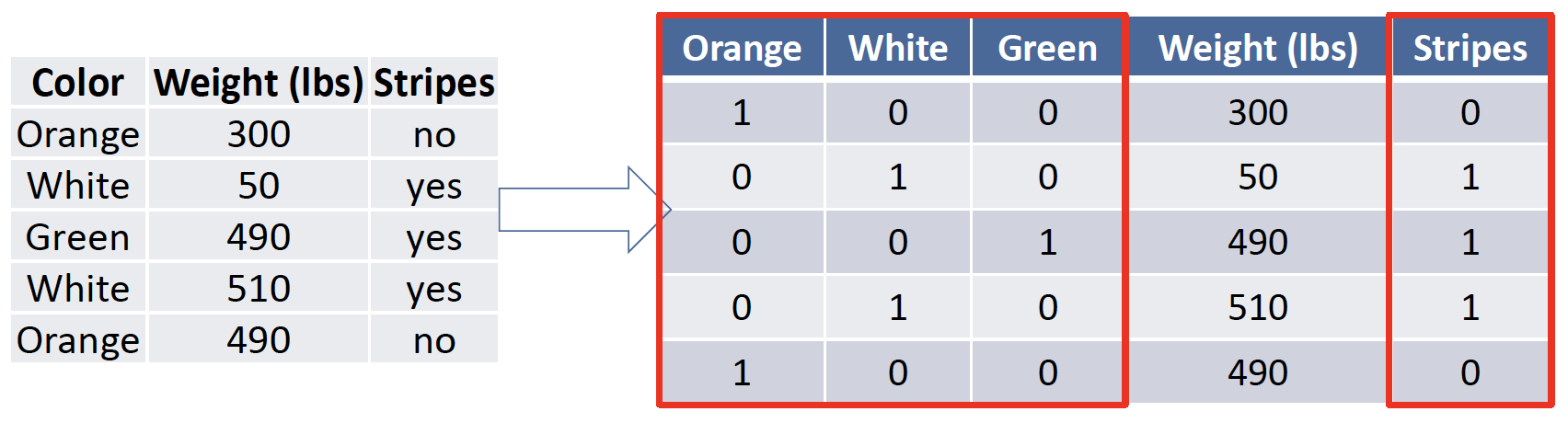
# KNN: Features must be numerical

Answer: Convert a categorical feature to binary features
将分类特征转换为二进制特征

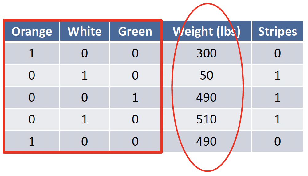
# KNN: Features must be normalized

Feature normalization is used to convert values in a feature to the same scales with values in other features.
特征归一化用于将特征中的值转换为与其他特征中的值相同的比例。

Answer: Yes, normalization is required, otherwise, the distance calculation will be influenced by the larger features!!!!
答：是的，需要归一化，否则，距离计算将受到较大特征的影响！

Min-max normalization: transformation from OldValue to NewValue
最小 - 最大标准化：从 OldValue 到 NewValue 的转换

$$\text { NewValue }=\text { NewMin }+\frac{\text { OldValue }-\text { OldMin }}{\text { OldMax }-\text { OldMin }} \times(\text { NewMax }-\text { NewMin })$$

# KNN: Overfitting Problem

• K value cannot be too small => overfitting!
  K 值不能太小 => 过拟合！
  You make decisions based on a small neighborhood
  根据一个小的邻里关系做决定
  It is possible to have bias in the model!
  模型中可能存在偏差！
• K value cannot be too large => underfitting!
  K 值不能太大 => 欠拟合！
  You make decisions based on a large neighborhood
  根据一个大的邻里关系来做决定的
• How to find the best K?
  如何找到最好的 K？
  • Try different K values in your experiments
    在实验中尝试不同的 K 值
    Do not always try 1, 3, 5, …, consider size of the data
    不要总是尝试 1、3、5，…，考虑数据的大小
    数据量大的话不需要从小的 K 值开始
  • Evaluate them in the correct strategy, and observe classification performance
    以正确的策略评估它们，并观察分类性能

# KNN: Learning Process?

• KNN is a lazy learned. There are no learning process
  KNN 是一个懒惰学习者。没有学习过程
• A learning process must have optimizations or loss functions
  学习过程必须具有优化或损失函数
• In KNN, we do not have optimization objective and methods. => machine learning
  在 KNN 中，我们没有优化目标和方法。=> 机器学习

# Summary

• K Nearest Neighbor (KNN) Classifier
  A simple classifier, a lazy learner

  1. Choose an odd number for K
  2. Calculate distances between target and instances in training set
  3. Pick the top KNN and assign the majority label as prediction

• Extended Problems in Classification Algorithms
  Q1. required data types?
  Q2. Is there an overfitting problem?
  Q3. Is there a learning process?

Note: they are general concerns in classification, not only KNN.

KNN Classifier

• Lazy classifier 懒惰分类
• Have to specify the value of K (cannot be too small or large) 必须指定 K 值，不能太小或太大
• Cannot handle categorical data, have to transform data 不能处理标称型数据，必须转换数据

# Naïve Bayes Classifier 朴素贝叶斯

• It is a probabilistic learning process
  这是一个概率学习过程
  • It is a simple classification algorithm too
    也是一种简单的分类算法
  • You should have some preliminary knowledge about probability
    应该有一些关于概率的初步知识
  • There are some requirements to use the Naïve Bayes classifier
    使用朴素贝叶斯分类器有一些要求

# Basic Concepts In Probability 概率论的基本概念

# $P(A \mid B)$

$P(A \mid B)$ is the probability of A given B; conditional probability
$P(A \mid B)$ 是 A 给定 B 的概率；条件概率

There are 10 examples here.
A: tiger = yes
B: color = orange

$$P(A) = 4/10 = 0.4$$

$$P(B) = 5/10 = 0.5$$

$$P(A \mid B) = 1/5$$

A 给定 B，假设 B 为 true 时 A 也为 true 的概率
先看 B color = orange 共有 5 条，再看同事满足 A tiger = yes 的只有 1 条

# $P(A \wedge B)$

Assumes that B is all and only information known.
假设 B 是所有且唯一已知的信息。

Defined by:

$$P(A \mid B)=\frac{P(A \wedge B)}{P(B)}$$

Bayes’s Rule: Direct corollary of above definition
贝叶斯法则：上述定义的直接推论

$$\begin{array}{l} P(A \wedge B)=\frac{P(A \mid B)}{P(A)}=P(B \wedge A)=\frac{P(B \mid A)}{P(B)} \\ \Rightarrow P(A \mid B)=\frac{P(A) P(B \mid A)}{P(B)} \end{array}$$

# $P\left(E \mid c_{i}\right)$

• Let set of classes be $\left\{c_{1}, c_{2}, \ldots c_{n}\right\}$, e.g., $c_{1} = tiger$ , $c_{2} = lion$
• Let $E$ be description of an example (e.g., a vector with feature values)
  设$E$ 是一个例子的描述 (例如，具有特征值的向量)
• Determine class of $E$ by computing for each class $c_{i}$
  通过计算每个类$c_{i}$ 来确定$E$ 的类（贝叶斯法则）

$$P\left(c_{i} \mid E\right)=\frac{P\left(c_{i}\right) P\left(E \mid c_{i}\right)}{P(E)}$$

• $P(E)$ can be determined since classes are complete and disjoint:
  Probability E $P(E)$ 可以确定，因为类是完整且不相交的：

$$\sum_{i=1}^{n} P\left(c_{i} \mid E\right)=\sum_{i=1}^{n} \frac{P\left(c_{i}\right) P\left(E \mid c_{i}\right)}{P(E)}=1$$

$$P(E)=\sum_{i=1}^{n} P\left(c_{i}\right) P\left(E \mid c_{i}\right)$$

Note: E is a feature vector, instead of a single feature!!
E 是特征向量，而不是单个特征！！
For example:
c: tiger = yes
E: color = orange, weight = 500 lbs, stripes = yes

$$E=e_{1} \wedge e_{2} \wedge \cdots \wedge e_{m}$$

$e_{1}$ 可以表示 color，$e_{2}$ 表示 weight，以此类推
m 表示 multiply，有多个特征

• Assume features are independent given the class ($c_{i}$), conditionally independent;
  假定特征给定类 ($c_{i}$) 是独立的，条件独立
  Therefore, we then only need to know $\mathrm{P}\left(e_{j} \mid c_{j}\right)$ for each feature and category IMPORTANT Assumption!!![IMPORTANT Assumption!!!]
  因此，我们只需要知道每个特征和类别的$\mathrm{P}\left(e_{j} \mid c_{j}\right)$【重要假设】

  $$P\left(E \mid c_{i}\right)=P\left(e_{1} \wedge e_{2} \wedge \cdots \wedge e_{m} \mid c_{i}\right)=\prod_{j=1}^{m} P\left(e_{j} \mid c_{i}\right)$$

在真实世界中，很难有好的统计学方法来验证特征和标签是否真的可以条件独立
只需要假设它们是有条件独立的，就可以使用此公式

# Conditional Independence

• $X$ is conditionally independent of $Y$ given $Z$, if the probability distribution for $X$ is independent of the value of $Y$, given the value of $Z$
  如果$X$ 的概率分布与$Y$ 的值无关，则$X$ 在给定$Z$ 的情况下有条件地独立于$Y$
• Generally, $P(X, Y \mid Z)=P(X \mid Z) \times P(Y \mid Z)$

Example 1

Let's say you flip two regular coins:

• A - Your first coin flip is heads
• B - Your second coin flip is heads
• C - Your first two flips were the same

Q1: What is the relationship between A and B?
Independent. Because the result of the first coin could not affect the result of second coin.

Q2: How about [A and B] by given C?
假设 C 是真的，那么 A 和 B 之间的依赖关系是什么
Dependent. Because the C told you that the result for the two coins, they are the same. If it is true, and if we know the result of A definitely, we know the result B.
This example is called conditionally dependent.

Example 2

There are a regular coin and a fake one (two heads)
有一枚普通硬币和一枚假硬币（两个头）
I randomly choose one of them and toss it twice
我随机选择其中一个，扔两次

• A - Your first flip is heads
• B - Your second flip is heads
• C - Your select a regular coin

Q1: What is the relationship between A and B?
Independent. Here I have two coins. I choose one of them and try to toss it twice. so in this case, I don't know which coin are selected. So probably I select a regular coin, probably I select a fake coin. The result for the first toss and second toss are independent.

Q2: How about [A and B] by given C?
Independent. Because C told you that you have a regular coin. If you select a regular coin, you toss it at one time, toss it two time. So the result of first time cannot affect the result for the second time. so this is called conditionally independent.

# Example

• c1: tiger = yes; c2: tiger = no
• E: e1: color = orange, e2: weight = 500 lbs, e3: stripes = yes

$$P(c_{1} \mid E)=\frac{P(c_{1}) P(E \mid c_{1})}{P(E)}$$

$$P(E \mid c_{1})=\prod_{j=1}^{m} P\left(e_{j} \mid c_{1}\right)$$

$$\begin{array}{l} P(e_{1} \mid c_{1})=1 / 4=0.25 \\ P(e_{2} \mid c_{1})=3 / 4=0.75 \\ P(e_{3} \mid c_{1})=4 / 4=1 \\ P(E \mid c_{1})=0.25 * 0.75 * 1=0.1875 \end{array}$$

$$\begin{array}{l} P(e_{1} \mid c_{2})=4 / 6=0.667 \\ P(e_{2} \mid c_{2})=1 / 6=0.167 \\ P(e_{3} \mid c_{2})=2 / 6=0.333 \\ P(E \mid c_{2})=0.667*0.167*0.333=0.0371 \end{array}$$

$$P(E)=\sum_{i=1}^{n} P\left(c_{i}\right) P\left(E \mid c_{i}\right)$$

$$\begin{array}{l} P(c_{1})=4 / 10=0.4 \\ P(c_{2})=6 / 10=0.6 \\ P(E)=P(c_{1}) P(E \mid c_{1})+P(c_{2}) P(E \mid c_{2})=0.09726 \\ P(c_{1} \mid E)=0.4 * 0.1875 / 0.09726=0.7711 \end{array}$$

$$P(c_{2} \mid E)=\frac{P(c_{2}) P(E \mid c_{2})}{P(E)}$$

$$P(c_{2} \mid E)=0.6 * 0.0371 / 0.09726=0.2289$$

$$P(c_{1} \mid E)>P(c_{2} \mid E)$$

We have more confidence to say we should trust $c_{1}$
更有信心说应该信任c_

In other words, $E$ should be classified as tiger!!!!
换句话说，$E$ 应该被归类为老虎！

It is very useful. A list of applications:

• Medical Detection: Given the situation of patients (such as cough, headache, body temp, etc ), make a decision he or she is in disease or not.
  医疗检测：根据患者的情况 (如咳嗽、头痛、体温等)，判断是否患病。
• Gender Classification: Given weights, age, heights, size of feet to judge a person is male or female
  性别分类：根据体重，年龄，身高，脚的大小来判断一个人是男性还是女性
• Social Robots: Given use behaviors on social networks, such as how many posts, how many friends, whether they use real human icons, the daily frequency of posts or friends, to make a decision this account is a real one or a fake one
  社交机器人：根据社交网络上的使用行为，比如有多少帖子，有多少好友，他们是否使用真人图标，每天发帖的频率或好友的频率，来决定这个账号是真的还是假的
• Text Classification : such as news or email classification
  文本分类：例如新闻或电子邮件分类

# General Questions for Classifications

• What are the required data types by an algorithm
• Is there an overfitting problem?
• Is there a training learning process?

# Naïve Bayes: Categorical Only 仅限标称型变量

Convert Numerical ones to categorical ones 把数值型转换成标称型

Numerical Features

Weights = 500
Weights > 500
Create two groups

# Naïve Bayes: Overfitting

• The overfitting issue is alleviated in Naïve Bayes, due to its nature probabilistic model using priori probabilities
  由于朴素贝叶斯使用先验概率的自然概率模型，过度拟合问题得到缓解

• But it may suffer from imbalance issue significantly
  但它可能会受到不平衡问题的严重影响

# Imbalance issue 不平衡问题

• It is a general issue in classification
  这是分类中的一个普遍问题
• It is not an issue in Naïve Bayes only
  这不仅仅是朴素贝叶斯的问题
• The issue: imbalance knowledge associated with labels in the training set
  问题：与训练集中的标签相关的不平衡知识
• Example
  • 100 examples, 60 are positive, 40 are negative
    100 例，60 例阳性，40 例阴性
  • 100 examples, 90 are positive, 10 are negative
    100 例，90 例阳性，10 例阴性
• Solutions: assume we have more positive samples
  解决方案：假设我们有更多的阳性样本
  • Undersampling [lose information, final data is small]
    欠采样 丢失信息，最终数据较小
    Remove some positive samples in the training
    删除训练集中的一些阳性样本
    Try to obtain a balance between positives & negatives
    尝试在正面和负面之间取得平衡
  • Oversampling [may result in overfitting]
    过采样 可能导致过拟合
    Replicate and add more negative data into training
    复制并将更多负面数据添加到训练中
    Try to obtain a balance between positives & negatives
    尝试在正面和负面之间取得平衡

Examples

• 100 examples, 95 are positives, 5 are negatives
  100 个例子，95 个是阳性，5 个是阴性

• Data split: training 83, testing 17
  数据分割：训练 83，测试 17
  In training set, 80 are positives, 3 are negatives
  在训练集中，80 个是阳性，3 个是阴性

• Solutions: assume we have more positive samples
  解决方案：假设我们有更多的阳性样本

  • Undersampling [lose information, final data is small]
    低度取样 [损失信息，最终数据很小］
    Use only 3 positives & 3 negatives in training set
    在训练集中只使用 3 个阳性和 3 个阴性样本
  • Oversampling [may result in overfitting]
    过度取样 [可能导致过度拟合] 。
    Use 80 positives and 80 negatives in training set
    在训练集中使用 80 个阳性和 80 个阴性样本
    Replicate the 3 negatives to have 80 negatives
    复制 3 个阴性，以获得 80 个阴性

These solutions can only apply on training data set here
这些解决方案只能适用于这里的训练数据集
apply this sampling of the whole data set, then try to split data.
对整个数据集应用这种抽样，然后尝试分割数据。
That's not correct. You should split data first.
这是不正确的。你应该先分割数据。
Then try to double check whether you have an imbalance issue on your training data set.
然后尝试仔细检查你的训练数据集是否有不平衡的问题。
If yes, you should apply undersampling or oversampling on the training data set only.
如果是，你应该只在训练数据集上应用欠采样或过采样。
Don't change test data set.
不要改变测试数据集。

# Special Issue in Naïve Bayes

• Violation of Independence Assumption
  违反独立性假设

  • It may be different to examine the assumptions
    检验这些假设可能会有所不同
  • Nevertheless, naïve Bayes works surprisingly well anyway!
    尽管如此，朴素贝叶斯的效果出人意料地好！

• Zero conditional probability Problem
  零条件概率问题

  • If no example contains the attribute value, i.e, $P\left(e_{1} \mid c\right)=0$
    如果没有示例包含属性值
  • In this circumstance, $P\left(E \mid c\right)=0$ will be zero too during test
    在这种情况下，$P\left(E \mid c\right)=0$ 在 test 期间也将为零

    $$P\left(E \mid c_{i}\right)=P\left(e_{1} \wedge e_{2} \wedge \cdots \wedge e_{m} \mid c_{i}\right)=\prod_{j=1}^{m} P\left(e_{j} \mid c_{i}\right)$$

  • For a remedy, conditional probabilities estimated with Laplace smoothing
    使用拉普拉斯平滑估计的条件概率，作为补救措施

    $$P\left(e_{i}=A \mid C=c_{j}\right)=\left(n_{c}+m * p\right) /(n+m)$$

    • $A$ is a value in the $i$-th feature;
      $A$ 是第$i$ 个特征中的值；
    • $c_{j}$ is a value in the label
      $c_{j}$ 是标签中的值
    • $\mathrm{n}_{\mathrm{c}}=\#$ of training instances for which $e_{i} = A$ and $C = c_{j}$.
      $\mathrm{n}_{\mathrm{c}}=\#$ 个训练实例，其中 $e_{i}=A$ 和 $C=c_{j}$。
    • $n = \#$ of training instances for which $C = c_{j}$.
      $n=\#$ 个训练实例，其中 $C=c_{j}$。
    • $m$ = a weight factor, usually $m>=1$ and could be big value, for example, the size of your training data
      $m$ = 权重因子，通常为$m>=1$，可以是很大的值，例如，训练数据的大小
    • $p$ = an estimate or a probability value to decrease $m$, usually, we can set $p$ as $1/t$ and $t$ is the number of unqiue values in $e_{i}$
      $p$ = 减少$m$ 的估计值或概率值，通常，我们可以将$p$ 设为$1/t$，$t$ 是$e_{i}$ 中唯一值的个数

  Note: it is only applied to the $P\left(e_{1} \mid c\right)$ component when it has the zero probability issue
  注意：当$P\left(e_{1} \mid c\right)$ 组件存在零概率问题时，它仅适用于该组件

# Summary

• Naïve Bayes is a probabilistic classification model
  朴素贝叶斯是一种概率分类模型
• It has one assumption: features are conditionally independent with labels
  它有一个假设：特征与标签有条件地独立
• Naïve Bayes Classification 朴素贝叶斯分类
  • Require categorical features 需要分类特征
  • Overfitting is not serious 过度拟合不严重
  • There is no learning process, but it may suffer from imbalance issue seriously
    虽然没有学习过程，但可能会出现严重的不平衡问题
  • Special issue: zero probability issue 零概率问题
    Solution: Laplace smoothing 解决方案：拉普拉斯平滑

Naïve Bayes Classifier

• Assumption: conditionally independent
  假设：条件独立
• Cannot handle numeric, have to transform data
  不能处理数值型，必须转换数据
• May have serious imbalance issues in labels (general issue in classification)
  标签可能存在严重的不平衡问题 (一般分类问题)

# Classification Evaluation Metrics 分类评价指标

# Accuracy is not the only metric

准确性不是唯一的衡量标准

Take binary classification for example
以二分分类为例

Confusion Matrix 混淆矩阵

$$\text { Accuracy }=\frac{T P + T N}{All}$$

$$\text { Error rate }=\frac{F P + F N}{All}$$

They are just overall metrics
它们只是总体指标

It is possible that a model works well on overall, but very bad on a single label
一个模型可能在整体上运行良好，但在单个标签上运行非常糟糕

Overall Acc = 90%, Acc on Positive label = 40%

# metric on positives & negatives

1. Precision 精确性
   exactness - what % of tuples that the classifier predicted as positive are positive
   精确度 - 分类器预测为正的元组中有多少百分比为正

   $$\text { precision }=\frac{T P}{T P+F P}$$

   TP + FP = total number of predicted as positives
   TP+FP = 预测为阳性的总数

2. Recall 召回率
   completeness what % of positive tuples did the classifier label as positive?
   完整性 - 分类器将多少百分比的正元组标记为正？

   $$\text { recall }=\frac{T P}{T P+F N}$$

   TP + FN = total number of actual positives
   TP+FN = 实际阳性总数

3. F measure (F1 or F score) F 度量
   harmonic mean of precision and recall
   精确性和召回率的调和平均值

   $$F=\frac{2 \times \text { precision } \times \text { recall }}{\text { precision }+\text { recall }}$$

4. Sensitivity 灵敏度
   True Positive recognition rate
   真阳性识别率

   $$\text { Sensitivity } = \frac{T P}{T P+F N} = \text { recall }$$

5. Specificity 特异性
   True Negative recognition rate
   真阴性识别率

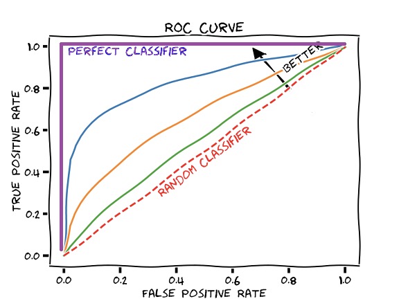
   $$\text { Specificity } = \frac{T N}{F P+T N}$$

6. ROC Curve ROC 曲线
   false positive vs true positive rate
   假阳性率与真阳性率
   false positive rate = 1 specificity
   假阳性率 = 1 特异性

   You can observe the AUC (area under the curve).
   可以观察曲线下的区域。
   If this area is larger, a model is better.
   这个区域越大，模型越好。
   In this case, the purple line is the best. the area and the curve is 100%.

• In real practice, reporting an overall metric is not enough.
  在实际操作中，仅报告总体指标是不够的。
  It is better to have the following combinations
  最好有以下几种组合

  • Model 1: acc = 80%, acc_1 = 80%, acc_0 = 80%
  • Model 2: acc = 80%, acc_1 = 95%, acc_0 = 70%
    在这个例子里，更倾向于使用 Model 1
    Because Model 2, even if the overall accuracy are the same, but the performance of different labels are not balanced.
    Model 2 即使整体精度与 Model 1 相同，但不同标签的性能并不均衡。

• Overall metric + metric on positives & negatives

  • Acc/Err + Precision/Recall/F1 + Specificity
  • Acc/Err + ROC
    用了 ROC，其他指标可以不用

# In-Class Practice

Calculate accuracy, err rate, precision, recall and F1, sensitivity and specificity for the following example
计算以下示例的准确率、错误率、精确度、召回率和 F1、敏感度和特异度