# Feature Selection and Reduction 特征选择与约简

• This is very important process in data analytics and data mining.

• Reason why?

  • Not all of the features are useful
    并非所有要素都有用
  • I rrelevant features will decrease accuracy
    相关要素会降低精确度
  • Data collection is an expensive process, you cannot simply remove features with your common sense
    数据收集是一个昂贵的过程，不能简单地根据常识移除要素
  • You must remove features or reduce dimensions by specific reasons
    必须基于特定原因移除要素或缩减维度

# Major Techniques of Dimensionality Reduction 降维的主要技巧

# Feature Selection 特征选择

Definition

A process that chooses an optimal subset of features according to a objective function
根据目标函数选择最佳特征子集的过程

Objectives

• To reduce dimensionality and remove noise
  降低维数并去除噪声
• To improve mining performance
  提高挖掘性能
  • Speed of learning
    学习速度
  • Predictive accuracy
    预测精度
  • Simplicity and comprehensibility of mined results
    挖掘结果的简单性和可理解性

Output 输出

Only a subset of the original features are selected
只有一个子集的原始特性

Feature Selection

• Filtering approach Kohavi and John, 1996
• Wrapper approach Kohavi and John, 1996
• Embedded methods I.Guyon et. al., 2006

# Feature Extraction/Reduction 特征提取 / 约简

Feature reduction

• refers to the mapping of the original high-dimensional data onto a lower-dimensional space
  特征约简是指将原始的高维数据映射到低维空间
• Given a set of data points of $p$ variables $\{ x_{1}, x_{2}, \dots x_{n} \}$
  Compute their low-dimensional representation:
  计算它们的低维表示:

  $$x_{i} \in \mathfrak{R}^{d} \rightarrow y_{i} \in \mathfrak{R}^{p}(p<<d)$$

Criterion

• Criterion for feature reduction can be different based on different problem settings.
  基于不同的问题设置，特征约简的标准可以不同。
• Unsupervised setting: minimize the information loss, e.g., PCA
  无监督设置：最小化信息损失
• Supervised setting: maximize the class discrimination, e.g., LDA
  监督设置：最大化阶级歧视

Input

All original features are used
所有原始功能

Output

The transformed features are linear combinations of the original features
变换后的要素是原始要素的线性组合

Dimensionality Reduction

• Principal Components Analysis (PCA)
• Nonlinear PCA (Kernel PCA, CatPCA)
• Multi Dimensional Scaling (MDS)
• Homogeneity Analysis

# Feature Selection 特征选择

# Components In Feature Selection

• For every feature selection technique, there must be at least two components
  对于每种特征选择技术，必须至少有两个组成部分
  • Quality Measure
    质量测量
  • Search/Rank Methods
    搜索 / 排名方法

# Example: Linear Regression

• In linear regression, we are going to predict a numerical variable $y$, by using a set of $x$ variables, e.g., $x_{1}, x_{2}, x_{3}, \dots , x_{n}$
  在线性回归中，我们将通过使用一组$x$ 变量来预测数值变量$y$

• Search Methods

  • Backward Elimination 反向消除
    Use all $x$ variables to build the model
    使用所有$x$ 变量来构建模型，
    Drop $x$ variables step by step to see whether we can improve the model
    逐步删除$x$ 变量，看看我们是否可以改进模型

  • Forward Selection 正向选择
    Build a simple model, e.g., a model with only one $x$
    构建一个简单的模型，例如，只有一个$x$ 的模型
    Try to add more $x$ variables step by step to see whether we can improve the model
    尝试逐步添加更多的$x$ 变量，看看我们是否可以改进模型

  • Stepwise = Forward + Backward 向前 + 向后

• In linear regression, we discuss different ways to select independent variables to predict the dependent variable
  在线性回归中，我们讨论了选择自变量来预测因变量的不同方法

  Search or Rank Method 搜索 / 排名方法 ---- Quality Measures 质量测量

  • Backward Elimination by using p-value
    利用 p 值反向消除
  • Backward Elimination by using AIC/BIC
    利用 AIC/BIC 反向消除
  • Forward Selection or Stepwise by using AIC/BIC
    使用 AIC/BIC 正向选择或逐步选择

# Quality Measure 质量测量

• The goodness of a feature/feature subset is dependent on measures
  特征 / 特征子集的优点取决于测量

• Various measures

  • Information measures (Yu & Liu 2004, Jebara & Jaakkola 2000)
  • Distance measures (Robnik & Kononenko 03, Pudil & Novovicov 98)
  • Dependence measures (Hall 2000, Modrzejewski 1993)
  • Consistency measures (Almuallim & Dietterich 94, Dash & Liu 03)
  • Accuracy measures (Dash & Liu 2000, Kohavi&John 1997)

# Information Measures

• Entropy of variable $X$ 变量$X$ 的熵

  $$H(X)=-\sum_{i} P\left(x_{i}\right) \log _{2}\left(P\left(x_{i}\right)\right)$$

  Impurity Measure 杂质测量

• Entropy of $X$ after observing $Y$ 观测$Y$ 后$X$ 的熵

  $$H(X \mid Y)=-\sum_{j} P\left(y_{j}\right) \sum_{i} P\left(x_{i} \mid y_{j}\right) \log _{2}\left(P\left(x_{i} \mid y_{j}\right)\right)$$

• Information Gain 信息增益

  $$I G(X \mid Y)=H(X)-H(X \mid Y)$$

This measure is used in decision tree classification
该测量用于决策树分类

# Accuracy Measures 准确度测量

• Using classification accuracy of a classifier as an evaluation measure
  使用分类器的分类精度作为评估指标

• Factors constraining the choice of measures
  限制措施选择的因素

  • Classifier being used
    正在使用的分类器
  • The speed of building the classifier
    构建分类器的速度

• Compared with previous measures 与之前的措施相比

  • Directly aimed to improve accuracy
    直接旨在提高准确性
  • Biased toward the classifier being used
    偏向于正在使用的分类器
  • More time consuming
    更耗时

# Feature Search 特征搜索

# Feature Ranking 特征排序

• Weighting and ranking individual features
  对单个特征进行加权和排序
• Selecting top ranked ones for feature selection
  选择排名靠前的特征
• Advantages
  • Efficient: $O(N)$ in terms of dimensionality $N$
  • Easy to implement
    易于实现
• Disadvantages
  • Hard to determine the threshold
    很难确定阈值
  • Unable to consider correlation between features
    不能考虑特征之间的相关性

# Two Models of Feature Selection

Filter model 过滤器模型

• Separating feature selection from classifier learning
  从分类器学习中分离特征选择
• Relying on general characteristics of data (information, distance, dependence, consistency)
  依赖于数据的一般特征 (信息、距离、依赖性、一致性)
• No bias toward any learning algorithm, fast running
  对任何学习算法都没有偏见，快速运行
  

Wrapper model 包装器模型

• Relying on a pre-determined classification algorithm
  依赖于预先确定的分类算法
• Using predictive accuracy as goodness measure
  使用预测精度作为优度测量
• High accuracy, computationally expensive
  高精度，计算成本高
  

# Feature Reduction 特征约简

# Feature Reduction Algorithms

• Unsupervised

  • Latent Semantic Indexing LSI : truncated SVD
  • Independent Component Analysis ICA
  • Principal Component Analysis PCA
  • Manifold learning algorithms

• Supervised

  • Linear Discriminant Analysis LDA
  • Canonical Correlation Analysis CCA
  • Partial Least Squares PLS

• Semi-supervised

Linear Discriminant Analysis LDA 线性判别分析

tries to identify attributes that account for the most variance between classes.
试图找出能够解释类之间差异最大的属性。
In particular, LDA , in contrast to PCA , is a supervised method, using known class labels.
特别是， LDA 相对于 PCA ，是一种有监督的方法，使用已知的类标签。

Principal Component Analysis PCA 主成分分析

applied to this data identifies the combination of linearly uncorrelated attributes (principal components, or directions in the feature space) that account for the most variance in the data.
应用于这些数据，来识别线性不相关属性 (主成分，或特征空间中的方向) 的组合，这些属性解释了数据中最大的差异。
Here we plot the different samples on the 2 first principal components.
这里我们把不同的样本绘制在两个第一主成分上。

Singular Value Decomposition SVD 奇异值分解

is a factorization of a real or complex matrix.
是实矩阵或复矩阵的因式分解。
Actually SVD was derived from PCA .
实际上， SVD 是从 PCA 中衍生出来的。

# Principal Component Analysis 主成分分析

# Schemes

Assume we have a data with multiple features
假设我们有一个具有多个特征的数据

1. Try to find principle components(PCs) each component is a combination of the linearly uncorrelated attributes/features;
   尝试寻找主成分 (PCs) 每个成分是线性不相关的属性 / 特征的组合
2. PCA allows to obtain an ordered list of those components that account for the largest amount of the variance from the data;
   PCA 允许从数据中获得解释最大方差的那些组件的排序列表；
3. The amount of variance captured by the first component is larger than the amount of variance on the second component, and so on.
   第一个组件捕获的差异量大于第二个组件的差异量，依此类推。
4. Then, we can reduce the dimensionality by ignoring the components with smaller contributions to the variance.
   然后，我们可以通过忽略对方差贡献较小的分量来降低维数。
5. The final reduced features we have are no longer the original features, but the difference PCs, each PC is a linear combination of your original features.
   我们最终减少的功能不再是原始功能，而是不同的 PCs，每台 PCs 都是原始功能的线性组合。

# How to obtain those principal components? 如何获得这些主成分？

The basic principle or assumption in PCA is:
主成分分析的基本原理或假设是：

The eigenvector of a covariance matrix equal to a principal component, because the eigenvector with the largest eigenvalue is the direction along which the data set has the maximum variance.
协方差矩阵的特征向量等于主成分，因为具有最大特征值的特征向量是数据集具有最大方差的方向。

Each eigenvector is associated with a eigenvalue;
每个特征向量都与一个特征值相关联；

Eigenvalue ➡️ tells how much the variance is;
特征值➡️代表方差有多大；

Eigenvector ➡️ tells the direction of the variation;
特征向量➡️代表变化的方向；

The next step: how to get the covariance matrix and how to calculate the eigenvectors/eigenvalues?
下一步：如何获得协方差矩阵以及如何计算特征向量 / 特征值？

# Visualization of PCA 可视化

The original expression by 3 genres is projected to two new dimensions, Such two dimensional visualization of the samples allow us to draw qualitative conclusions about the separability of experimental conditions (marked by different colors).
原来的三种类型的表达式被投影到两个新的维度，这种样本的二维可视化允许我们对实验条件 (用不同的颜色标记) 的可分性得出定性的结论。

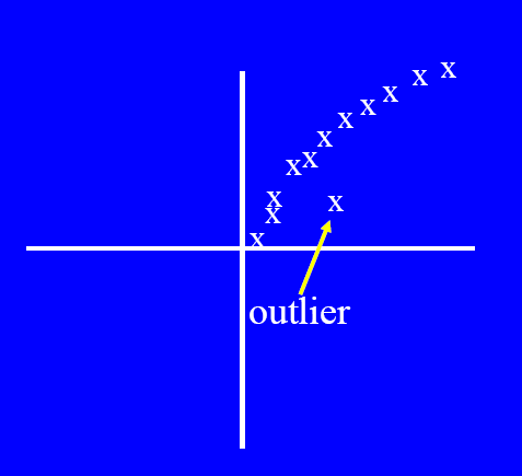
# Anomaly/Outlier Detection 异常 / 离群值检测

• What are anomalies/outliers? 什么是异常 / 离群值

  • The set of data points that are considerably different than the remainder or the majority of the data
    与剩余数据或大部分数据有很大差异的数据点集

• Variants of Anomaly/Outlier Detection Problems 异常 / 离群值检测问题的变体

  • Given a database D , find all the data points $x \in D$ with anomaly scores greater than some threshold t
    给定一个数据库 D ，在$x \in D$ 中查找异常分数大于某个阈值 t 的所有数据点
  • Given a database D , find all the data points $x \in D$ having the top-n largest anomaly scores $f(x)$
    给定一个数据库 D ，找出所有数据点$x \in D$ 的前 n 个最大异常得分$f(x)$
  • Given a database D , containing mostly normal (but unlabeled) data points, and a test point $x$ , compute the anomaly score of $x$ with respect to D
    给定一个数据库 D ，其中包含大部分正常（但未标记）数据点和一个测试点$x$，计算$x$ 关于 D 的异常分数

• Applications 应用

  • Credit card fraud detection 信用卡欺诈检测
  • telecommunication fraud detection 电信欺诈检测
  • network intrusion detection 网络入侵检测
  • fault detection 故障检测

# Anomaly Detection Schemes

• General Steps:
  一般步骤

  1. Build a profile of the “normal” behavior
     建立 “正常” 行为的轮廓

     • Profile can be patterns or summary statistics for the overall population
       轮廓可以是总体群体的模式或汇总统计数据

  2. Use the “normal” profile to detect anomalies
     使用 “正常” 轮廓检测异常

     • Anomalies are observations whose characteristics differ significantly from the normal profile
       异常是特征与正常轮廓显著不同的观察结果

• Types of anomaly detection schemes
  异常检测方案的类型

  • Graphical 图形
  • Model based 基于模型
  • Distance based 基于距离
  • Clustering based 基于聚类

# Graphical Approaches 图解法

Boxplot (1-D), Scatter plot (2-D), Spin plot (3-D)

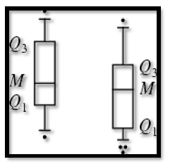
• Limitations 限制
  • Time consuming 耗时
  • Subjective 主观

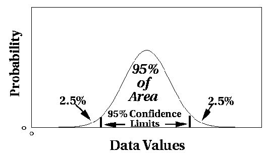
# Statistical Approaches - Model based 统计方法 - 基于模型

• Assume a parametric model describing the distribution of the data (e.g., normal distribution)
  假设参数模型描述数据的分布 (例如，正态分布)
• Apply a statistical test that depends on
  应用统计检验，该检验取决于
  • Data distribution
    数据分布
  • Parameter of distribution (e.g., mean, variance)
    分布的参数 (例如，均值、方差)
  • Number of expected outliers (confidence limit)
    预期离群值的数量 (置信极限)

# Distance-based Approaches 基于距离的方法

• Data is represented as a vector of features
  数据表示为要素矢量
• Three major approaches 三种主要方法
  • Nearest neighbor based 基于最近邻
  • Density based 基于密度
  • Clustering based 基于聚类

# Nearest-Neighbor Based Approach

• Compute the distance between every pair of data points
  计算每对数据点之间的距离
• There are various ways to define outliers:
  定义异常值的方法有多种：
  • Data points for which there are fewer than p neighboring points within a distance D
    距离 D 内邻接点少于 p 个的数据点
  • The top n data points whose distance to the kth nearest neighbor is greatest
    与第 k 个最近邻点的距离最大的前 n 个数据点
  • The top n data points whose average distance to the k nearest neighbors is greatest
    到 k 个最近邻域的平均距离最大的前 n 个数据点

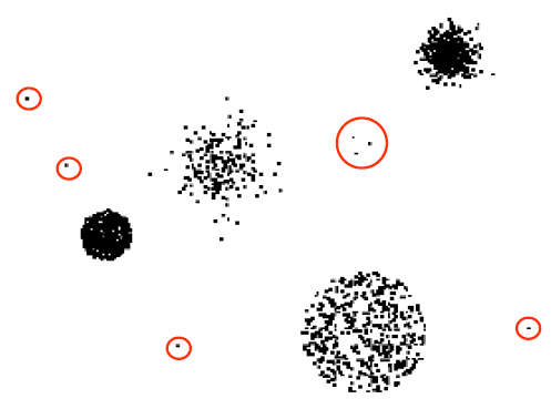
# Clustering-Based

• Idea: Use a clustering algorithm that has some notion of outliers!
  想法：使用具有离群值概念的聚类算法！
• The data which are far away from the centroid could be outliers
  远离质心的数据可能是离群值
• The set of data in a small cluster could be outliers
  一个小聚类中的数据集可能是离群值

# Density-based: LOF approach

• For each point, compute the density of its local neighborhood; e.g. use DBSCAN’s approach
  对于每个点，计算其局部邻域的密度；例如，使用 DBSCAN 的方法
• Compute local outlier factor (LOF) of a sample p as the average of the ratios of the density of sample p and the density of its nearest neighbors
  计算样本 p 的局部异常值因子 (LOF) 为样本 p 的密度与其最近邻域的密度之比的平均值
• Outliers are points with largest LOF value
  离群值是 LOF 值最大的点

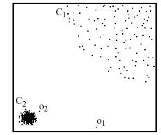
In the NN approach, $o_{2}$ is not considered as outlier, while LOF approach find both $o_1$ and $o_{2}$ as outliers
在神经网络方法中，$o_{2}$ 不被认为是异常值，而 LOF 方法发现$o_{1}$ 和$o_{2}$ 都是异常值

• Alternative approach: directly use density function; e.g. DENCLUE’s density function
  另一种方法：直接使用密度函数，例如登克莱密度函数