# Decision Trees 决策树
「机器学习实战」摘录 - 决策树
k - 近邻算法可以完成很多分类任务,但是它最大的缺点就是无法给出数据的内在含义,决策树的主要优势就在于数据形式非常容易理解。
决策树算法能够读取数据集合,决策树的一个重要任务是为了数据中所蕴含的知识信息,因此决策树可以使用不熟悉的数据集合,并从中提取出一系列规则,在这些机器根据数据集创建规则时,就是机器学习的过程。
专家系统中经常使用决策树,而且决策树给出结果往往可以匹敌在当前领域具有几十年工作经验的人类专家。
- 优点:计算复杂度不高,输出结果易于理解,对中间值的缺失不敏感,可以处理不相关特征数据。
- 缺点:可能会产生过度匹配问题。
- 适用数据类型:数值型和标称型。
# Basic
A decision tree is a flow chart like tree structure
决策树是一个类似树状结构的流程图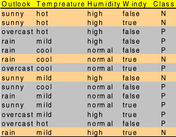
# How it works?
- We learn and build a tree structure based on the training set
我们基于训练集学习并构建一个树结构 - After that, we are able to make predictions based on the tree
然后,我们能够基于树进行预测 - Example, Is it good to play golf? {sunny, windy, high humidity}
适合打高尔夫吗? 晴朗、多风、高湿度 - Question: How to learn such a tree? There could be many possible trees
问题:如何学习这样的树?可能有许多可能的树
Example: “is it a good day to play golf?”
a set of attributes and their possible values
- outlook → sunny, overcast, rain
- temperature → cool, mild, hot
- humidity → high, normal
- windy → true, false
In this case, the target class is a binary attribute, so each instance represents a positive or a negative example.
在本例中,目标类是一个二进制属性,因此每个实例表示一个正示例或一个负示例。
- So a new instance:
<rainy ,hot, normal, true>: ?
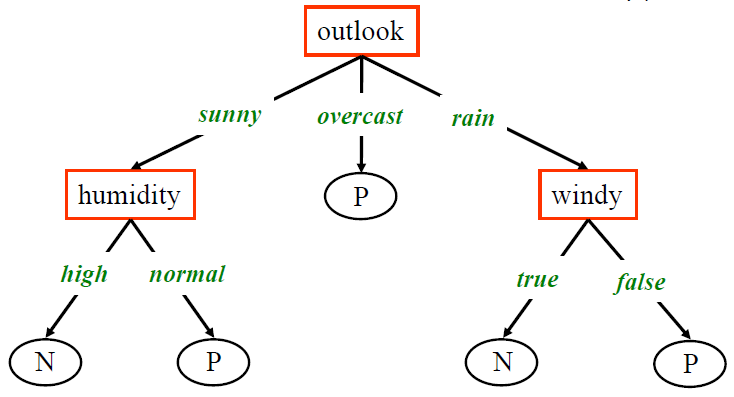
will be classified as "noplay"- Root node: the top of the tree, e.g. the node
Outlook
根节点 - Parent and Children nodes:
outlookas the parent,humidityandwindyare children nodes
outlook 作为父节点,“湿度” 和 “风象” 是子节点 - Leaf node:
P,Nare the leaf nodes which do not have children and we can reach a leaf node to get the predictionsP,N是没有子节点的叶节点,我们可以到达叶节点来获得预测
- Root node: the top of the tree, e.g. the node
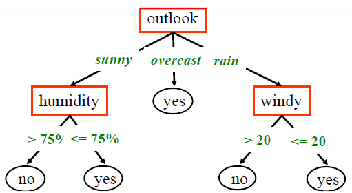
- If attributes are continuous, it should be converted into a nominal variable
如果属性是连续型变量,则应将其转换为标称型变量- Each path in the tree represents a decision rule:
- Rule1:
If (outlook="sunny") AND (humidity <= 0.75) Then (play="yes") - Rule2:
If (outlook="rainy") AND (wind > 20) Then (play="no") - Rule3:
If (outlook="overcast")
Then (play="yes")
- Rule1:
- Each path in the tree represents a decision rule:
# Popular Tree Based Learning Techniques 流行的基于树的学习技术
- ID3
- or Iternative Dichotomizer, was the first of these three Decision Tree techniques implementations developed by Ross Quinlan (Quinlan, J. R. 1986. Induction of Decision Trees. Mach. Learn. 1, 1 (Mar. 1986), 81-106.)
或 Iternative Dichotomizer,是这三种决策树技术的第一个实现,由 Ross Quinlan 开发 - C4.5
- Quinlan's next iteration. 昆兰的下一个迭代。
The new features (versus ID3) are:
新的特征(相对于 ID3)是
1. accepts both continuous and discrete features;
同时接受连续和离散的特征。
2. handles incomplete data points;
处理不完整的数据点。
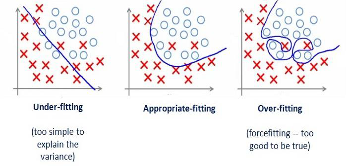
3. solves over-fitting problem by (very clever) bottom-up technique usually known as "__pruning__"; and
通过(非常聪明的)自下而上的技术解决过度拟合问题,通常被称为 "剪枝";以及
4. different weights can be applied the features that comprise the training data.
可以对组成训练数据的特征使用不同的权重。
- CART
- or Classification And Regression Trees. 或分类和回归树。
The CART implementation is very similar to C4.5; the one notable difference is that CART constructs the tree based on a numerical splitting criterion recursively applied to the data.
CART 的实现与 C4.5 非常相似;一个明显的区别是,CART 是根据一个递归应用于数据的数字分割标准来构建树。
# Top-Down Decision Tree Generation 自上而下的决策树生成
The basic approach usually consists of two phases:
基本方法通常包括两个阶段:- Tree construction 树的构建
- At the start, all the training examples are at the root
开始时,所有的训练实例都在根部 - Partition examples are recursively based on selected attributes
根据选定的属性,递归地分割实例
- At the start, all the training examples are at the root
- Tree pruning 树的修剪
- remove tree branches that may reflect noise in the training data and lead to errors when classifying test data
删除可能反映训练数据中的噪声并导致测试数据分类时出现错误的树枝 - improve classification accuracy
提高分类精度
- remove tree branches that may reflect noise in the training data and lead to errors when classifying test data
- Tree construction 树的构建
Basic Steps in Decision Tree Construction 决策树构建的基本步骤
- Tree starts a single node representing all data
树开始是一个代表所有数据的单一节点 - If sample are all same classthen node becomes a leaf labeled with class label
如果样本都是同一类别,那么节点就会成为标有类别标签的叶子。 - Otherwise, select feature that best separates sample into individual classes.
否则,选择最能将样本分成各个类别的特征。 - Recursion stops when:
递归在以下情况下停止:- Samples in node belong to the same class (majority)
节点中的样本属于同一类别(多数)。 - There are no remaining attributes on which to split
没有剩余的属性可供分割
- Samples in node belong to the same class (majority)
- Tree starts a single node representing all data
# Feature Selection 特征筛选
Choosing the “Best” Feature
- Feature selection 特征筛选
- is the key component in decision trees: deciding what features of the data are relevant to the target class we want to predict.
是决策树的关键部分:决定数据的哪些特征与我们要预测的目标类别相关。
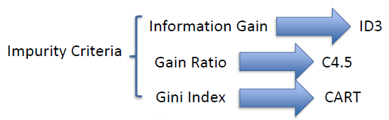
- Popular impurity measures in decision tree learning
决策树学习中流行的杂质度量- Information Gain: Used in ID3.
信息增益。在 ID3 中使用。 - Gain Ratio: improvement over information gain. It is used in C4.5
增益比:对信息增益的改进。它在 C4.5 中使用 - Gini Index: Used in CART. It is a measure of how often a randomly chosen element from the set would be incorrectly labelled if it was randomly labelled according to the distribution of labels in the subset.
吉尼指数。在 CART 中使用。它是衡量从集合中随机选择的元素,如果按照子集合中的标签分布随机贴上标签,那么它被错误贴上标签的频率。
- Information Gain: Used in ID3.
# Understand Entropy & Information Gain 理解熵和信息增益
The decision tree is built in a top down fashion, but the question is how do you choose which attribute to split at each node?
决策树是自顶向下构建的,但问题是如何选择在每个节点上分割哪个属性?
The answer is find the feature that best splits the target class into the purest possible children nodes ( ie : nodes that don't contain a mix of both male and female, rather pure nodes with only one class ).
答案就是找到能够最好地将目标类分解为尽可能纯的子节点的特性 (例如:不包含男性和女性混合的节点,而是只包含一个类的纯节点)。For instance, in our previous example on recognition of tigers and lions, we have features like stripes, weights, size, color , etc. But, you may notice that, “stripes” is the key feature to distinguish tigers and lions!
例如,在我们上一个关于老虎和狮子识别的例子中,我们有条纹、重量、大小、颜色等特征,但是,你可能会注意到,“条纹” 是区分老虎和狮子的关键特征!This measure of information is called purity.
这种对信息的衡量被称为纯净度。Entropy is a measure of impurity. Information Gain which is the difference between the entropies before and after.
熵是对不纯度的一种衡量。信息增益,是前后熵的区别。Information_Gain = Entropy_before split - Entropy_after split
信息增益 = 分割前的熵 - 分割后的熵Entropy_before split = Impurity before the split
分割前的熵 = 分割前的不纯度Entryopy_after split = Impurtiy after the split
分割后的熵 = 分割后的不纯度The larger an information gain value (by a feature) is, the feature should be used to split the instances as the “best” node.
一个信息增益值(由一个特征决定)越大,该特征应该被用来作为 "最佳" 节点来分割实例。
# Trees Construction Algorithm (ID3)
# Decision Tree Learning Method (ID3)
Input: a set of training examples , a set of features
- If every element of has a class value “yes”, return “yes”; if every element of S has class value “no”, return “no”
- Otherwise, choose the best feature from (if there are no features remaining, then return failure);
- Extend tree from by adding a new branch for each attribute value of
- Set
- Distribute training examples to leaf nodes (so each leaf node represents the subset of examples of with the corresponding attribute value
- Repeat steps 1-5 for each leaf node with as the new set of training examples and as the set of attributes until we finally label all the leaf nodes
Main Question:
- how do we choose the best feature at each step?
Note: ID3 algorithm only deals with categorical attributes, but can be extended (as in C4.5) to handle continuous attributes
# Choosing the “Best” Feature
Use Information Gain to find the “best” (most discriminating) feature
- Assume there are two classes, and (e.g, = “yes” and = “no”)
- Let the set of instances (training data) contains elements of class and elements of class
- The amount of information, needed to decide if an arbitrary example in belongs to or is defined in terms of entropy, :
- Note that
- More generally, if we have classes, and are the number of instances of in each class, then the entropy is:
where is the probability that an arbitrary instance belongs to the class
- Now, assume that using attribute a set of instances will be partitioned into sets each corresponding to distinct values of attribute .
- If contains cases of and cases of , the entropy, or the expected information needed to classify objects in all subtrees is
$$\operatorname{Pr}\left(S_{i}\right)=\frac{\left|S_{i}\right|}{|S|}=\frac{p_{i}+n_{i}}{p+n}$$The probability that an arbitrary instance in belongs to the partition S_
- If contains cases of and cases of , the entropy, or the expected information needed to classify objects in all subtrees is
- The encoding information that would be gained by branching on
We use attribute to split node = Entropy before splitting - Entropy after splitting by using feature
- At any point we want to branch using an attribute that provides the highest information gain.
# Attribute Selection - Example


# Other Criteria
Information Entropy and Information Gain
it is used in ID3Drawbacks of Information Gain
- If an attribute has large number of values, it is more possible to be pure by using this attribute
- IG will introduce biases for these attributes which have large number of values
- The bias will further result in overfitting problem
Gain Ratio
- It was first introduced to C4.5 classification
- It was first introduced to C4.5 classification
Gini Index
- It was used in the CART algorithm
Same questions in Decision Trees:
- Any data requirements?
Categorical data can be used directly; numeric data may be transformed to categorical ones. Numeric data can be automatically utilized or transformed in C4.5- Is there a learning/optimization process
Yes, we are going to learn a tree structure.- Overfitting in DT?
More details in the next page.
# Overfitting and Pruning
# Overfitting Problem
- Problem: The model is over-trained by the training set; it may showa high accuracy on training set, but significantly worse performance on test set.
- Let’s see an example
- You worked classifications on a data set. The data set is big, so you used hold-out evaluation.
You build a model based on training, and evaluate the model based on the testing set.
Finally, you get a 99% classification accuracy on the testing set. Is this an example of overfitting? - How about N-fold cross validations?
- You worked classifications on a data set. The data set is big, so you used hold-out evaluation.

- Overfitting in DT: A tree may obtain good results on training, but bad on testing
- The tree may be too specific with many branches & leaf nodes
# Solution: Tree Pruning
- A tree generated may over-fit the training examples due to noise or too small a set of training data
- Two approaches to alleviate over-fitting:
- Stop earlier: Stop growing the tree earlier
- Post-prune: Allow over-fit and then post-prune the tree
- Example of the Stop-Earlier:
- Examine the classification metric (such as accuracy) at each node. Stop the splitting process if the metric meets pre-defined value
- Use Minimum Description Length
MDLprinciple: halting growth of the tree when the encoding is minimized.
# Post-Pruning the Tree
- A decision tree based on the training data may need to be pruned
- over-fitting may result in branches or leaves based on too few examples
- pruning is the process of removing branches and subtrees that are generated due to noise; this improves classification accuracy
- Subtree Replacement: merge a subtree into a leaf node
- At a tree node, if the accuracy without splitting is higher than the accuracy with splitting, replace the subtree with a leaf node; label it using the majority class
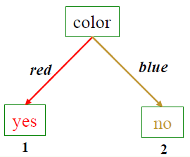
Suppose with test set we find 3 red “no” examples, and 2 blue “yes” example. We can replace the tree with a single “no” node. After replacement there will be only 2 errors instead of 5.
Summary
| KNN Classifier | Naive Bayes Classifier | Decision Trees | |
|---|---|---|---|
| Principle | Find the KNN by distances; Assign the major class label; | Calculate conditional probability; compare probability of each label given an example | "Build a tree by top-down fashion. The node is selected by""best"" feature" |
| Assumptions | No | Features are conditional independent with labels | No |
| Feature Types | Categorical data should be converted to binary values | Numeric va lues may be converted to categorical ones | Numeric values may be converted to categorical ones |
| Feature Normalization | Yes | No | No |
| Overfitting | Lazy learner; Parameters | Imbalance classes | Tree Pruning |
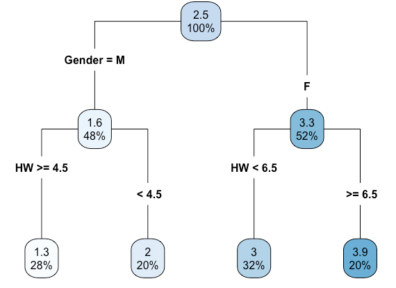
# Regression Tree
- Decision tree, by default, was developed for classifications where the target variable is a nominal variable
- The tree-based method can also be extended to predict or estimate a numerical variable – it is the technique of Regression Tree
- To further understand regression tree, let’s compare decision classification tree vs regression tree
| Regression Tree | Classification Tree | |
|---|---|---|
| Target variable | Nominal | Numerical |
| Output in Leaf | Nominal label | Numerical value (mean of set) |
| Impurity | G or Gini index | MSE (mean squared error) |
| Branches | Could be more than two | Binary |
| Comparison between classification trees and regression trees | ||
# How it works
How to split the space to create branch/trees
Everytime, it iterates all possible value or categories in each feature to create a binary split
The impurity is MSE. We want to find the best split which makes lowest MSE in each split
We continue the splitting until it meets stopping criteriaHow to output a numerical value in leaf node
The value is the mean of values in a splitted group
Tree Based Learning
- More complicated but much more effective sometimes
更复杂,但有时更有效- Tree based learning: a machine learning method
基于树的学习:一种机器学习方法- Require feature selection
需要特征选择- Require to handle overfitting problems (Stop Earlier or Post Pruning)
要处理过拟合问题 (提前停止或后期剪枝)
# Logistic Regression Logistic 回归
「机器学习实战」摘录 - Logistic回归
利用 Logistic 回归进行分类的主要思想是:根据现有数据对分类边界线建立回归公式,以此进行分类。
这里的 “回归” 一词源于最佳拟合,表示要找到最佳拟合参数集。
训练分类器时的做法就是寻找最佳拟合参数,使用的是最优化算法。
- 优点:计算代价不高,易于理解和实现。
- 缺点:容易欠拟合,分类精度可能不高。
- 适用数据类型:数值型和标称型数据。
- Both Logistic regression and Linear SVM model can be considered as linear classification models.
Logistic 回归模型和线性 SVM 模型都可以视为线性分类模型。
They tried to utilize linear models to solve the problem of classifications
试图利用线性模型来解决分类问题 - We discuss logistic regression and SVM by using a binary classification as an example
以二分类为例讨论逻辑回归和 SVM - Note that both of them can be applied to multi class classifications too
这两种方法也可以应用于多类分类
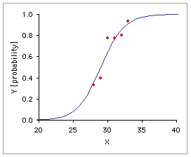
# Simple Logistic regression model 简单 Logistic 回归模型
Relationship between qualitative binary variable Y and one x-variable:
定性二元变量 Y 和一个 x 变量之间的关系:
Model for probability for each value .
对于每个值 的概率 的模型。
measures the odds that event occurs
测量 事件发生的概率
In logistic regression, we use 1 and 0 to denote binary labels
在逻辑回归中,用 1 和 0 来表示二进制标号
# Interpreting
Let the probability of “success”
设 成功的概率
- If odd>1 then ➔
- If odd=1 then ➔
- If odd<1 then ➔
# General Logistic Regression
- We may have several x variables in the model
模型中可能有几个 x 变量 - 0.5 is the default cut off value, but we may improve the model by using other cut off values
0.5 是默认的 cut off 值,但可以使用其他的 cut off 值来改进模型- ➔ predicted as 1
- ➔ predicted as 0
- Try different alpha values to see which one is the best
尝试不同的 alpha 值,看看哪个是最优的
- The model is interpretable. can be considered as a confidence value
模型是可解释的。 可以认为是一个置信度值
# Model fitting or building 模型拟合或建造
- The process is similar to the linear regression models
过程类似于线性回归模型 - X must be numerical variable. Transformation is required if there are nominal variables
X 必须是数值变量,如果有标称变量,则需要进行转换。 - Feature selection methods, such as backward elimination, forward or stepwise selection, can also be applied
特征选择方法,如向后消除,向前或逐步选择,也可以应用 - Residual analysis needs to be performed
需要进行残留分析 - The model is evaluated by classification metrics, such as accuracy, precision, recall, ROC curve, etc
通过准确率、精密度、召回率、ROC 曲线等分类指标对模型进行评价
# Example: Logistic Regression
Data: Case Study 3 Admissions
admit,gre,gpa,rank
0,380,3.61,3
1,660,3.67,3
1,800,4,1
1,640,3.19,4
0,520,2.93,4
1,760,3,2
1,560,2.98,1
0,400,3.08,2
load and split data
mydata = read.csv("case3_admission.csv", header=T)
mydata = mydata[sample (nrow (mydata)),]
select.data = sample(1:nrow (mydata), 0.8*nrow (mydata))
train.data = mydata[select.data,]
test.data = mydata[-select.data, ]
head(mydata)
    admit	gre	gpa	rank
265	1	520	3.90	3
140	1	600	3.58	1
120	0	340	2.92	3
172	0	540	2.81	3
247	0	680	3.34	2
168	0	720	3.77	3
train.label = train.data$admit
test.label = test.data$admit
build model by FS
full = glm(admit~gre+gpa+rank, data=train.data, family=binomial())
base = glm(admit~gpa, data=train.data, family=binomial())
library(leaps)
step(base, scope=list (upper=full, lower=~1), direction="both", trace=F)
Call: glm(formula = admit ~ gpa + rank + gre, family = binomial(), data=train.data)

Coefficients:
(Intercept)	gpa	rank	gre
-2.861669	0.683853	-0.594686	0.002019

Degrees of Freedom: 319 Total (i.e. Null); 316 Residual
Null Deviance:	402.1
Residual Deviance: 370.7	AIC:378.7
produce probabilities
prob = predict(full, type="response", newdata=test.data)
choose cut off value to calculate accuracy
for(i in l:length(prob)){
if(prob[i] > 0.5) { # cut off value
prob[i] = l
} else {
prob[i] = 0
}}library(Metrics)
accuracy(test.label, prob)
[1] 0.6875for(i in l:length(prob)){
if(prob[i] > 0.4) { # cut off value
prob[i] = l
} else {
prob[i] = 0
}}[1] 0.7
「机器学习实战」摘录 - Logistic回归的一般过程
- 收集数据:采用任意方法收集数据。
- 准备数据:由于需要进行距离计算,因此要求数据类型为数值型。另外,结构化数据格式则最佳。
- 分析数据:采用任意方法对数据进行分析。
- 训练算法:大部分时间将用于训练,训练的目的是为了找到最佳的分类回归系数。
- 测试算法:一旦训练步骤完成,分类将会很快。
- 使用算法:首先,我们需要输入一些数据,并将其转换成对应的结构化数值;接着,基于训练好的回归系数就可以对这些数值进行简单的回归计算,判定它们属于哪个类别;在这之后,我们就可以在输出的类别上做一些其他分析工作。
# Support Vector Machines (SVM) 支持向量机
「机器学习实战」摘录 - 支持向量机
有些人认为,SVM 是最好的现成的分类器,这里说的 “现成” 指的是分类器不加修改即可直接使用。同时,这就意味着在数据上应用基本形式的 SVM 分类器就可以得到低错误率的结果。SVM 能够对训练集之外的数据点做出很好的分类决策。
- 优点:泛化错误率低,计算开销不大,结果易解释。
- 缺点:对参数调节和核函数的选择敏感,原始分类器不加修改仅适用于处理二类问题。
- 适用数据类型:数值型和标称型数据。
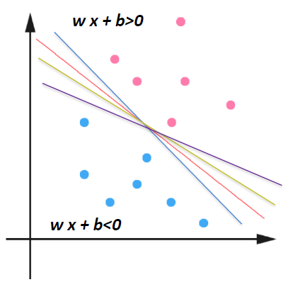
# Linear SVM
- Draw a linear model to separate two classes
画一个线性模型来区分两个类
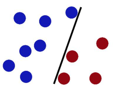
- The model could be a straight line model (such as regression line in 2D space)
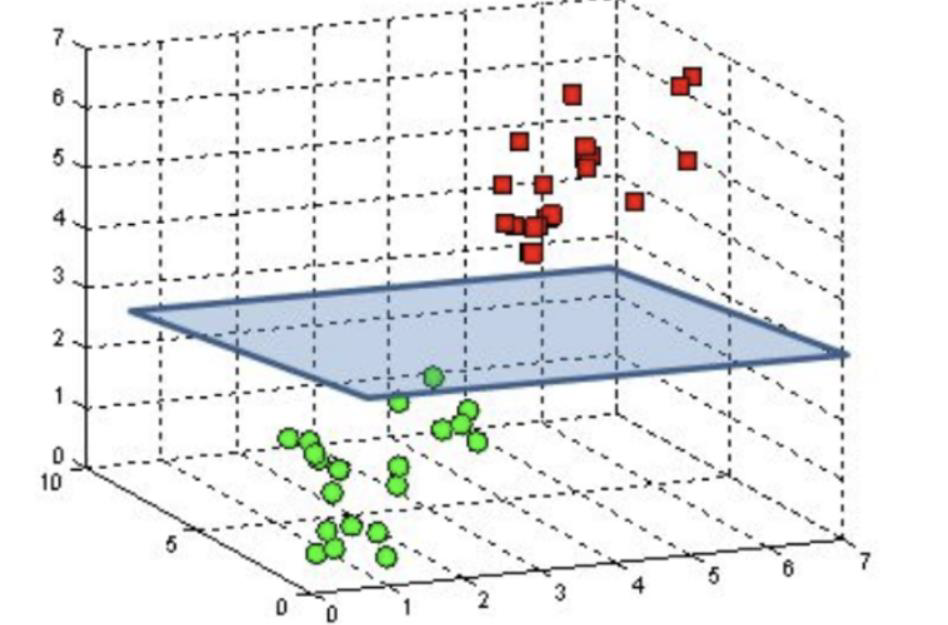
模型可以是直线模型 (如二维空间中的回归线) - The model could be a hyperplane model in multi dimensional space
模型可以是多维空间中的超平面模型
We use straight line model as an example in the class. But, you should also keep in mind that the hyperplane model is still linear SVM
课堂上以直线模型为例。但是还应该记住,超平面模型仍然是线性 SVM。
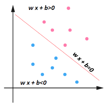
PINK denotes → +1
BLUE denotes → -1
In logistic regression, we use
0and1for binary labels.
在逻辑回归中,我们使用0和1作为二进制标签。
In SVM, we use+1and-1as binary labels.
在 SVM 中,我们使用+1和-1作为二进制标签。
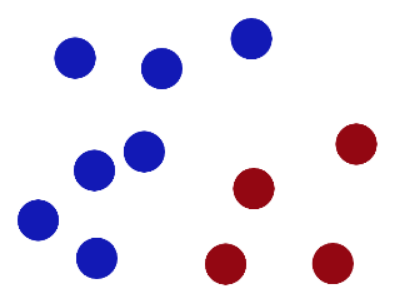
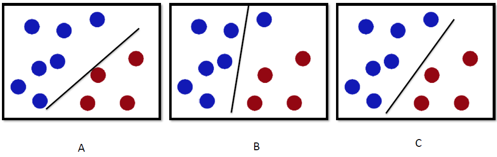
How would you classify this data?
Any of these would be fine..
「机器学习实战」摘录 - 超平面
上述将数据集分隔开来的直线称为分隔超平面 separating hyperplane 。
数据点都在二维平面上,此时分隔超平面就只是一条直线。
但是,如果所给的数据集是三维的,那么此时用来分隔数据的就是一个平面。
显而易见,更高维的情况可以依此类推。
如果数据集是 1024 维的,那么就需要一个 1023 维的某某对象来对数据进行分隔。
这个 1023 维的某某对象到底应该叫什么?N-1 维呢?
该对象被称为超平面 hyperplane ,也就是分类的决策边界。
分布在超平面一侧的所有数据都属于某个类别,而分布在另一侧的所有数据则属于另一个类别。
采用这种方式来构建分类器,即如果数据点离决策边界越远,那么其最后的预测结果也就越可信。
..but which is best?
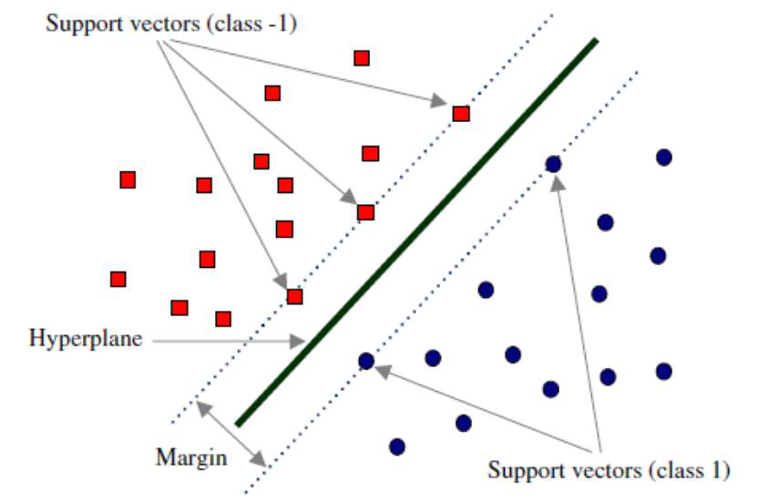
# Definition: Margin 间隔
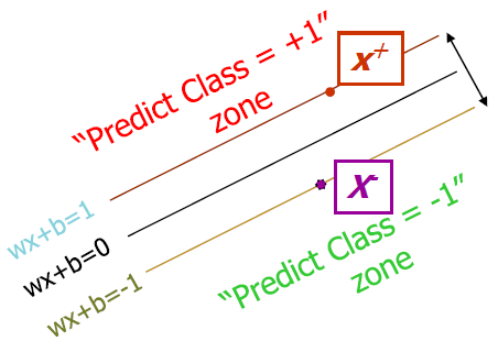
Define the hyperplane such that:
定义超平面 为:
and are the planes:
The points on the planes and are the points in two classes (+1, -1) on the boundary.
平面 和 上的点是边界上两类 (+1, -1) 中的点。
They are also called the Support Vectors.
它们也被称为支持向量。
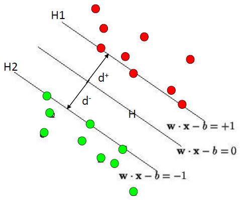
= the shortest distance to the closest positive point
到最近的正点的最短距离
= the shortest distance to the closest negative point
到最近的负点的最短距离
The margin of a separating hyperplane is
分隔超平面的边界是 。
set = Margin Width
Objective: Maximal Margin in SVM Classification
目的:支持向量机分类的最大边界
What we know:
「机器学习实战」摘录 - 间隔
我们希望找到离分隔超平面最近的点,确保它们离分隔面的距离尽可能远。
这里点到分隔面的距离被称为间隔 margin 。
我们希望间隔尽可能地大,这是因为如果我们犯错或者在有限数据上训练分类器的话,我们希望分类器尽可能健壮。
支持向量 support vector 就是离分隔超平面最近的那些点。
# Method: Maximizing the Margin 寻找最大间隔
We want a classifier with as big margin as possible.
Maximize ➔ Minimize ➔ Minimize = objective function 目标函数
「机器学习实战」摘录 - 寻找最大间隔
如何求解数据集的最佳分隔直线?先来看看图 6-3。
分隔超平面的形式可以写成 。
要计算点 A 到分隔超平面的距离,就必须给出点到分隔面的法线或垂线的长度,该值为 。
这里的常数 类似于 Logistic 回归中的截距。
这里的向量 和常数 一起描述了所给数据的分隔线或超平面。接下来我们讨论分类器。
# Solving the Optimization Problem 解决分类器求解的优化问题
Find and such that
is minimized;
and for all
Need to optimize a quadratic function subject to linear constraints.
需要优化一个受线性约束的二次函数。
Quadratic optimization problems are a well-known class of mathematical programming problems, and many (rather intricate) algorithms exist for solving them.
二次优化问题是一类著名的数学规划问题,有许多 (相当复杂的) 算法来解决它们。
The solution involves constructing a dual problem where a Lagrange multiplier associated with every constraint in the primary problem:
解决方案涉及构造一个对偶问题,其中拉格朗日乘子 与主问题中的每个约束相关联:
Find such that
is maximized and
- for all .
「机器学习实战」摘录 - 为什么SVM类别标签采用-1和+1,而不是0和1呢?
这是由于 -1 和 +1 仅仅相差一个符号,方便数学上的处理。
我们可以通过一个统一公式来表示间隔或者数据点到分隔超平面的距离,同时不必担心数据到底是属于 -1 还是 +1 类。
当计算数据点到分隔面的距离并确定分隔面的放置位置时,间隔通过 来计算,这时就能体现出 -1 和 +1 类的好处了。
被称为点到分隔面的函数间隔, 称为点到分隔面的几何间隔。
如果数据点处于正方向(即 +1 类)并且离分隔超平面很远的位置时, 会是一个很大的正数,同时 也会是一个很大的正数。
而如果数据点处于负方向( -1 类)并且离分隔超平面很远的位置时,此时由于类别标签为 -1 ,则 仍然是一个很大的正数。
「机器学习实战」摘录 - 找出分类器定义中的w和b
为此,我们必须找到具有最小间隔的数据点,而这些数据点也就是前面提到的支持向量。
一旦找到具有最小间隔的数据点,我们就需要对该间隔最大化。这就可以写作:
直接求解上述问题相当困难,所以我们将它转换成为另一种更容易求解的形式。
首先考察一下上式中大括号内的部分。
由于对乘积进行优化是一件很讨厌的事情,因此我们要做的是固定其中一个因子而最大化其他因子。
如果令所有支持向量的 都为 1,那么就可以通过求 的最大值来得到最终解。
但是,并非所有数据点的 都等于 1,只有那些离分隔超平面最近的点得到的值才为 1。
而离超平面越远的数据点,其 的值也就越大。
在上述优化问题中,给定了一些约束条件然后求最优值,因此该问题是一个带约束条件的优化问题。
这里的约束条件就是。
对于这类优化问题,有一个非常著名的求解方法,即拉格朗日乘子法。
通过引入拉格朗日乘子,我们就可以基于约束条件来表述原来的问题。
由于这里的约束条件都是基于数据点的,因此我们就可以将超平面写成数据点的形式。于是,优化目标函数最后可以写成:
尖括号表示 和 两个向量的内积
其约束条件为:
和
至此,一切都很完美,但是这里有个假设:数据必须 100% 线性可分。
# Dataset with noise
- Hard Margin
- So far we require all data points be classified correctly
到目前为止,我们要求所有的数据点都是正确分类的
No training errors are allowed
不允许有任何训练错误
Hard margin will build models without errors, which may introduce overfitting
硬边际将建立没有误差的模型,这可能会引入过拟合
- Soft Margin
- we allow errors but we want to minimize the errors
我们允许错误,但我们希望最小化错误
Soft margin allows errors in the model, which may help build a more general model
软边际允许模型中出现错误,这可能有助于建立一个更普遍的模型
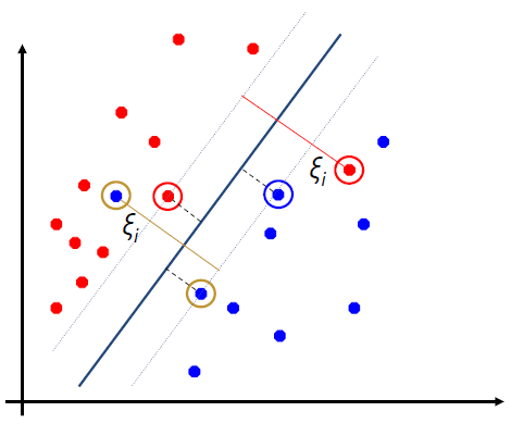
Slack variables can be added to allow misclassification of difficult or noisy examples.
可以增加松弛变量,以便对困难或有噪声的例子进行错误分类。![]()
New objective function Minimize 新目标函数最小化

The old formulation:
Hard Margin
Find and such that
is minimized;
and for all :The new formulation incorporating slack variables:
Soft Margin
Find and such that
is minimized;
and for all :
and for allParameter can be viewed as a way to control overfitting.
常数 可以被看作是一种控制过拟合的方法。
「机器学习实战」摘录 - 松弛变量(slack variable)
几乎所有数据都不那么 “干净”。
这时我们就可以通过引入所谓松弛变量 slack variable ,来允许有些数据点可以处于分隔面的错误一侧。
这样我们的优化目标就能保持仍然不变,但是此时新的约束条件则变为:
和
这里的常数 用于控制 “最大化间隔” 和 “保证大部分点的函数间隔小于 1.0” 这两个目标的权重。
在优化算法的实现代码中,常数 是一个参数,因此我们就可以通过调节该参数得到不同的结果。
一旦求出了所有的 ,那么分隔超平面就可以通过这些 来表达。
这一结论十分直接,SVM 中的主要工作就是求解这些 。
# Non-Linear SVM
Datasets that are linearly separable with some noise work out great:
带有一些噪声的线性可分数据集效果很好:![]()
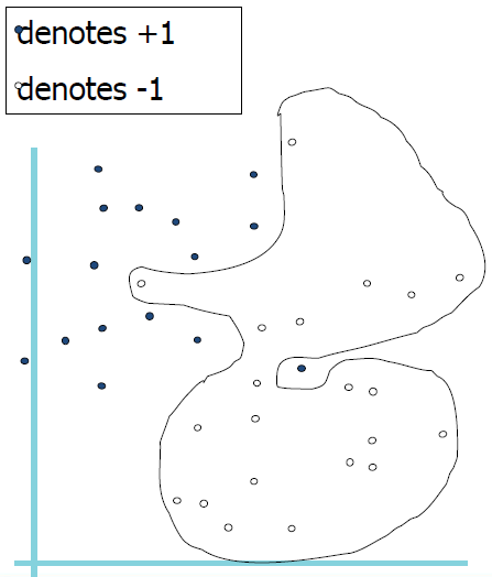
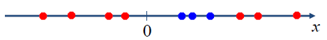
But what are we going to do if the dataset is just too hard?
![]()
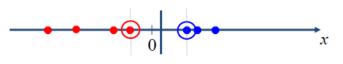
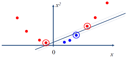
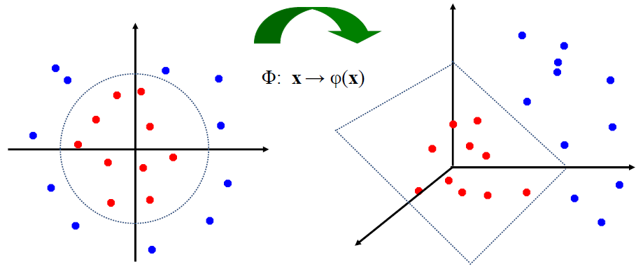
How about mapping data to a higher dimensional space:
把数据映射到更高维的空间如何:![]()
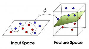
# Feature spaces 特征空间
We can map the original data to higher dimensional space
![]()
General idea: 总体思路:
the original input space can always be mapped to some higher-dimensional feature space where the training set is separable:
原始输入空间总是可以映射到某个训练集可分离的高维特征空间:![]()
In the 2D space, our linear SVM model is
在 2D 空间中,我们的线性 SVM 模型是In the MD space, our model becomes
are the new vectors mapped to a higher dimensional space
是映射到更高维度空间的新向量
# The Kernel Function 核函数
A Kernel Function is some function that corresponds to an inner product in some expanded feature space.
核函数是对应于某个扩展特征空间中的内积的函数。It helps us convert the input space from lower dimension to higher dimension by using the inner product.
它帮助我们利用内积将输入空间从低维转换到高维。
- Examples of Popular Kernel Functions
- Linear Kernel
- Polynomial Kernel of power p
- Gaussian (radial basis function network) Kernel
- Sigmoid Kernel
# Non-linear SVMs Mathematically
Dual problem formulation:
Find such that
is maximized and- for all .
The solution is: Still linear formula
- Optimization techniques for finding is remain the same!
# Overview
- SVM finds a separating hyperplane in the feature space and classify points in that space.
SVM 在特征空间中找到一个分离超平面,并对该空间中的点进行分类。 - It does not need to represent the space explicitly, simply by defining a kernel function.
它不需要显式地表示该空间,只需定义一个核函数。 - The kernel function plays the role of the dot product in the feature space.
核函数在特征空间中起点积的作用。
# Weakness of SVM
# It is sensitive to noise 它对噪音很敏感
A relatively small number of mislabeled examples can dramatically decrease the performance
相对较少的错误标记示例可能会显著降低性能
# It only considers two classes 它只考虑两类
how to do multi-class classification (MCC) with SVM?
如何用支持向量机进行多类分类?
There are many methods to convert MCC to binary classification.
有很多方法可以将 MCC 转换为二进制分类。
Below is one of these methods:
下面是其中一种方法:
with output arity m, learn m SVM’s
- SVM 1 learns
Output == 1vsOutput != 1 - SVM 2 learns
Output == 2vsOutput != 2 - ...
- SVM m learns
Output == mvsOutput != m
- SVM 1 learns
To predict the output for a new input, just predict with each SVM and find out which one puts the prediction the furthest into the positive region.
要预测新输入的输出,只需对每个 SVM 进行预测,并找出哪个预测最接近正区域。
# Support Vector Regression (SVR)
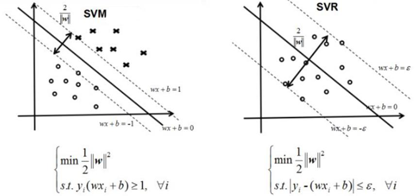
In SVM, we have two lines on the boundary -they are the lines closest to the hyper-plane (i.e., the SVM classifier line or plane). Our model is the hyper-plane which wants to maximize the margin/distances
在 SVM 中,我们在边界上有两条线 —— 它们是最接近超平面的线 (即 SVM 分类器线或平面)。我们的模型是超平面,它想要最大化余量 / 距离In SVR, we have two lines on the boundary -they are the lines farthest to the hyper-plane (i.e., the regression line). Our model is the hyper plane or regression line which minimizes the distances
在 SVR 中,我们在边界上有两条线 —— 它们是离超平面最远的线 (即回归线)。我们的模型是超平面或回归线,它使距离最小化Same characteristics: the hyper-plane are the models in between the boundary lines
相同的特征:超平面是边界线之间的模型
# Multi-Class Classification by Binary Classification 二元分类法的多类分类法
- All the classification techniques we discussed can be applied to multi class classifications
所有分类技术都可以应用于多类分类 - Multi Class classification can be solved by multiple binary classifications
多类分类可以通过多个二元分类来解决- One vs. One
- One vs. Rest
- Many vs. Many
# Strategy 1: One vs. One
- Assume we have labels
假设我们有 个标签 - We will choose unique pair of these labels, and perform binary classifications
我们将选择这些标签的唯一对,并执行 二进制分类 - We will get classification results
我们将得到 分类结果 - Finally, we use voting to get the final prediction results
最后,利用投票的方式得到最终的预测结果 - Notes: one label as positive, another as negative
注:一个标签是正的,另一个是负的
Example: Assume we have 4 labels: c1, c2, c3, c4
We will get unique pairs
| c1, c2 | Binary Classification | Predictions |
| c1, c3 | Binary Classification | |
| c1, c4 | Binary Classification | |
| c2, c3 | Binary Classification | |
| c2, c4 | Binary Classification | |
| c3, c4 | Binary Classification |
# Strategy 2: One vs. Rest
- Assume we have labels
假设我们有 个标签 - We will perform binary classifications
我们将执行 二进制分类 - In each classification, we predict vs. Not-
在每个分类中,我们预测 vs. Not- - Finally, we use voting to get the final prediction results
最后,利用投票的方式得到最终的预测结果 - Notes: one label as positive, others as negative
注:一个标签是正的,另一个是负的
Example: Assume we have 4 labels: c1, c2, c3, c4
We will perform binary classifications
| c1, ┐c1 | Binary Classification | Predictions |
| c2, ┐c2 | Binary Classification | |
| c3, ┐c3 | Binary Classification | |
| c4, ┐c4 | Binary Classification |
# Strategy 3: Many vs. Many
- Assume we have labels
假设我们有 个标签 - We will perform binary classifications
我们将执行 二进制分类 - They encode labels into new ones
它们将标签编码成新的标签 - Example: Error Correcting Output Codes, ECOC
- Notes: one set as positive, another set as negative
注:一组为正,另一组为负