# Objectives 目标
- Understand the difference between Point Estimate and Interval Estimate
了解点估计和区间估计的区别 - Know how to use R to construct a confidence interval on Mean/Proportion , Difference of Two Means/Proportions, Variance and Ratio of Variances
知道如何使用 R 构建均值 / 比例、两个均值 / 比例的差值、方差和方差比的置信区间
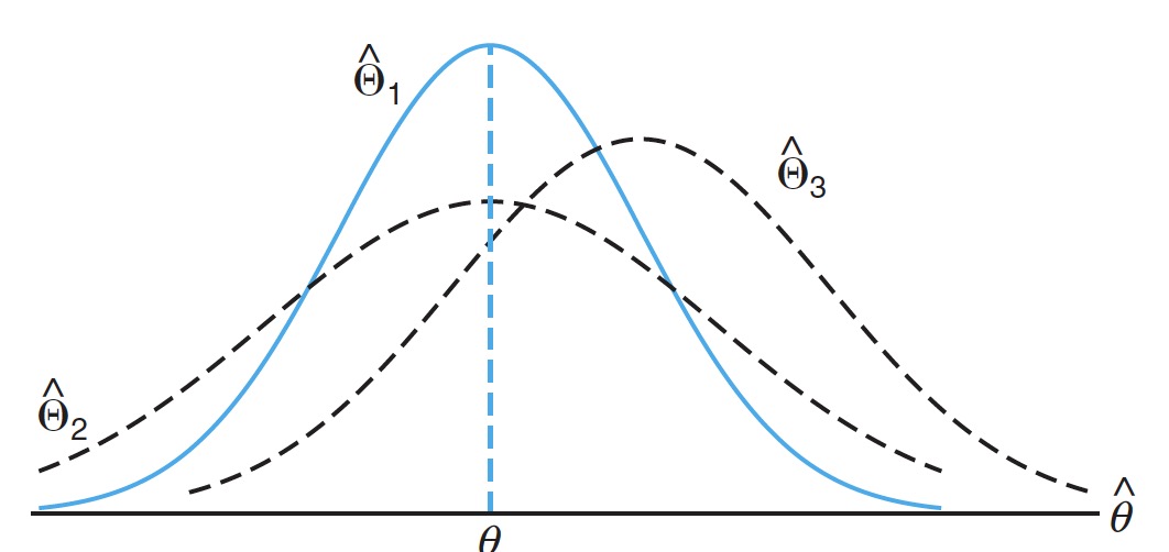
# Point Estimate (Not good) 点估计
# Generate standard normal random numbers with sample size 100 | |
samplesize<- 100 | |
normsample<- rnorm(samplesize) | |
mean(normsample) |
[1] 0.04918487
median(normsample) |
[1] 0.203471
var(normsample) |
[1] 1.020872
Let's increase the sample size to 10000
# Generate standard normal random numbers with sample size 10000 | |
samplesize<- 10000 | |
normsample<- rnorm(samplesize) | |
mean(normsample) |
[1] 0.005888358
median(normsample) |
[1] 0.005134332
var(normsample) |
[1] 0.9931025
Which point estimator is 'better'?
# Interval Estimate 区间估计
# Confidence Interval on when known 已知总体标准差 ,求均值 的置信区间
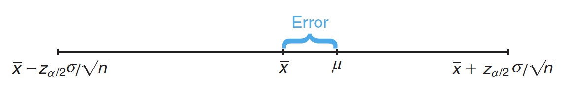
The interval contains the true population mean with probability 95%, where is the sample mean, is the sample size, and is population standard deviation.
区间 有 95% 的概率包含真实的总体均值,其中 是样本均值, 是样本大小, 是总体标准差。
- how was this calculated?
这是如何计算的? - what does the "95% probability" mean?
“95% 的概率” 是什么意思?
According to the Central Limit Theorem, we have is approximately normal distributed with mean and variance ,
根据中心极限定理,样本 取自总体均值为 ,总体方差为 的近似正态分布
i.e.,
Suppose denote the value such that
假设 表示
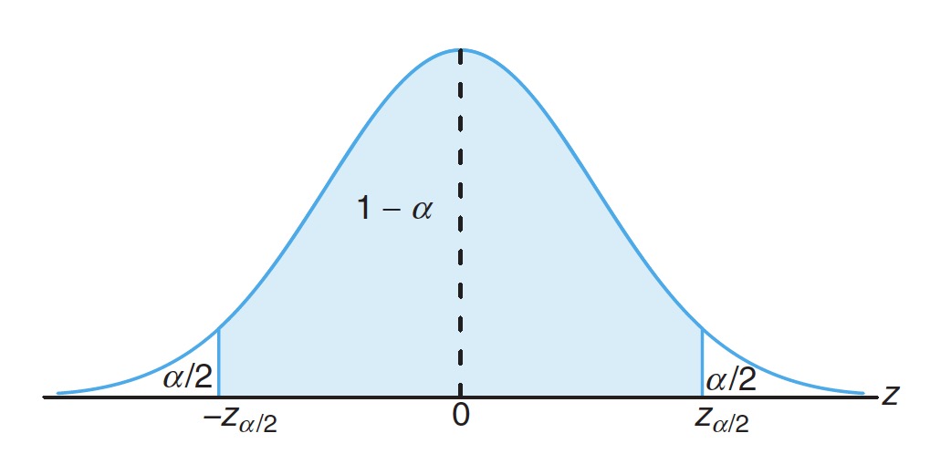
As confidence is 95%, we know , that is .
由于置信度为 95%,则 ,即 。
How to find ?
如何找到 ?
z_0.025 <- qnorm(0.975) # why? | |
z_0.025 |
[1] 1.959964
Why confidence interval better?
为什么置信区间更好?
The confidence interval provides an estimate of the accuracy of our point estimate.
置信区间提供了对点估计准确性的评价。
Question: How to construct 99% confidence interval?
如何构建 99% 置信区间?
# In-class Exercise: CI on with known variance 已知总体方差,求总体均值 的 置信区间
The average zinc concentration recovered from a sample of measurements taken in 36 different locations in a river is found to be 2.6 grams per milliliter.
从河流中不同位置的 36 个测量样本中回收的平均锌浓度为 2.6 克 / 毫升。
Find the 95% and 99% confidence intervals for the mean zinc concentration in the river.
找出河流中平均锌浓度的 95% 和 99% 置信区间。
Assume that the population standard deviation is 0.3 gram per milliliter.
假设总体标准偏差为 0.3 克 / 毫升。
n <- 36 | |
sigma <- 0.3 | |
xbar <- 2.6 | |
alpha <- 0.05 | |
loBound <- xbar - qnorm(1-alpha/2)*sigma/sqrt(n) | |
loBound |
[1] 2.502002
upBound <- xbar + qnorm(1-alpha/2)*sigma/sqrt(n) | |
upBound |
[1] 2.697998
alpha <- 0.01 | |
loBound <- xbar - qnorm(1-alpha/2)*sigma/sqrt(n) | |
loBound |
[1] 2.471209
upBound <- xbar + qnorm(1-alpha/2)*sigma/sqrt(n) | |
upBound |
[1] 2.728791
# Confidence Interval on when unknown 总体方差 未知,求总体均值 的置信区间
# If we don't know 如果不知道总体标准差 t-distribution
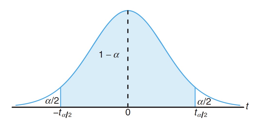
If the population follows normal distribution or approximately normal distribution, we can use distribution.
如果总体服从正态分布或近似正态分布,我们可以使用 分布。
If we have a random sample from a normal distribution, then the random variable
如果我们有一个来自正态分布的随机样本,那么随机变量
has a Student -distribution with degrees of freedom.
呈自由度为 的 Student 分布。
Here is the sample standard deviation.
这里 指样本标准差。
If and are the mean and the standard deviation of a random sample of size from a distribution with unknown variance , a confidence interval for is given by
如果大小为 的随机样本,样本均值为 、样本标准差为 ,取自具有未知总体方差 的正态分布总体,则总体均值 的 置信区间由下式给出
where is the value with degrees of freedom, leaving an area of to the right.
其中 表示 自由度为 、 右侧区域的 值。
# Example 1 t.test
The contents of seven similar containers of sulfuric acid are 9.8, 10.2, 10.4, 9.8, 10.0, 10.2, and 9.6 liters.
七个类似容器的硫酸容量分别为 9.8、10.2、10.4、9.8、10.0、10.2 和 9.6 升。
Find a 95% confidence interval for the mean contents of all such containers, assuming an approximately normal distribution.
假设总体近似正态分布,计算所有此类容器容量平均值的 95% 置信区间。
sulfruicAcid<-c(9.8,10.2,10.4,9.8,10.0,10.2,9.6) | |
xbar <- mean(sulfruicAcid) | |
s <-sd(sulfruicAcid) | |
n <- 7 | |
t6_0.025<- qt(0.975,n-1) | |
lowerBound <- xbar-t6_0.025*s/sqrt(n) | |
lowerBound |
[1] 9.738414
upperBound <- xbar+t6_0.025*s/sqrt(n) | |
upperBound |
[1] 10.26159
A different way to get confidence interval
获得置信区间的另一种方法
t.test(sulfruicAcid, conf.level = .95) |
    One Sample t-test

data:  sulfruicAcid
t = 93.541, df = 6, p-value = 1.006e-10
alternative hypothesis: true mean is not equal to 0
95 percent confidence interval:
  9.738414 10.261586
sample estimates:
mean of x
       10
# In-class Exercise: CI on with unknown variance 总体方差未知,求总体均值 的置信区间
Regular consumption of presweetened cereals contributes to tooth decay, heart disease, and other degenerative diseases, according to studies conducted by Dr. W. H. Bowen of the National Institute of Health and Dr. J. Yudben, Professor of Nutrition and Dietetics at the University of London.
一项研究,经常食用预先加糖的谷物会导致蛀牙、心脏病和其他退行性疾病。
In a random sample consisting of 20 similar single servings of Alpha-Bits, the average sugar content was 11.3 grams with a standard deviation of 2.45 grams.
在由 20 份类似的单份 Alpha-Bits 组成的随机样本中,平均含糖量为 11.3 克,标准偏差为 2.45 克。
Assuming that the sugar contents are normally distributed, construct a 95% confidence interval for the mean sugar content for single servings of Alpha-Bits.
假设糖含量呈正态分布,为单份 Alpha-Bits 的平均糖含量构建 95% 的置信区间。n <- 20
xbar <- 11.3
s <- 2.45
alpha <- 0.05
tvalue <- qt(1-alpha/2,df = n-1)
loBound <- xbar - tvalue *s/sqrt(n)
loBound
[1] 10.15336upBound <- xbar + tvalue *s/sqrt(n)
upBound
[1] 12.44664Please construct a 95% confidence interval for the mean of
Sepal.Lengthin theIrisdata set.
为Iris数据集中的Sepal.Length的均值构建 95% 的置信区间。t.test(iris$Sepal.Length)
 One Sample t-test

data:  iris$Sepal.Length
t = 86.425, df = 149, p-value < 2.2e-16
alternative hypothesis: true mean is not equal to 0
95 percent confidence interval:
 5.709732 5.976934
sample estimates:
mean of x
 5.843333
# Estimating the Difference between Two Means 评价两个均值之间的差异
Next, we want to investigate two populations with means and and variances and , respectively.
调查分别有均值 和,方差 和 的两个群体。
Thus we can have a point estimator of the difference between and is given by the statistic .
可以用统计量 表示 和 之间的差异。
# Confidence Interval on when and known 总体方差 和 已知时,求总体均值差异 的置信区间
If and are the means of independent random samples of sizes and from populations with known variances and , respectively, a confidence interval for is given by
如果大小 和 的独立随机样本的均值分别是 和 ,取自总体方差为 和 的两个总体,则总体均值差异 的 的置信区间为
where is the value leaving an area of to the right.
代表在 右侧区域取得的 值。
# Example 2
A study was conducted in which two types of engines, and were compared.
一项研究,比较 和 两种类型的发动机。
Gas mileage, in miles per gallon, was measured.
以英里 / 加仑为单位测量汽油里程。
Fifty experiments were conducted using engine type and 75 experiments were done with engine type .
型进行了 50 次实验, 型进行了 75 次。
The gasoline used and other conditions were held constant.
使用的汽油和其他条件保持不变。
The average gas mileage was 36 miles per gallon for engine and 42 miles per gallon for engine .
发动机的平均油耗为每加仑 36 英里。 发动机每加仑行驶 42 英里。
Find a 96% confidence interval on where and are population mean gas mileages for engines and , respectively.
分别是 的均值,找到 96% 的置信区间。
Assume that the population standard deviations are 6 and 8 for engines and , respectively.
假设 发动机的总体标准差分别为 6 和 8。
alpha <- 0.04 | |
n1 <- 50 | |
x1 <- 36 | |
n2 <- 75 | |
x2 <- 42 | |
sigma1 <- 6 | |
sigma2 <- 8 | |
standerror <- sqrt(sigma1^2 /n1 + sigma2^2/n2) | |
lowerBound <- x2-x1 - qnorm(1-alpha/2)*standerror | |
lowerBound |
[1] 3.42393
upperBound <- x2-x1 + qnorm(1-alpha/2)*standerror | |
upperBound |
[1] 8.57607
# In-class Exercise: CI on with known and 已知总体方差 和 ,求总体均值差异 的置信区间
Generate 50 normal random numbers with and and get the sample mean .
Hint:rnorm
从 和 的正态中生成 50 个随机数,并得到样本均值 。Generate 75 normal random numbers with and and get the sample mean
从 和 的正态中生成 75 个随机数,并得到样本均值 。Please construct a 95% confidence interval on .
请构建两个总体均值差异 的 95% 置信区间 。
x1<-rnorm(500,mean = 3, sd = 3) | |
x2<-rnorm(750,mean = 2, sd = 4) | |
x1bar <- mean(x1) | |
x2bar <- mean(x2) | |
standerr <- sqrt(3^2/500+4^2/750) | |
alpha <- 0.05 | |
zalpha2 <- qnorm(1-alpha/2) | |
loBound <- x1bar - x2bar -zalpha2*standerr | |
loBound |
[1] 0.9058725
upBound <- x1bar - x2bar + zalpha2*standerr | |
upBound |
[1] 1.683297
Question: If we don't know the variances, what should we do?
如果我们不知道方差,我们应该怎么做?
# Confidence Interval on when but Both Unknown 已知 但两者都未知,求 的置信区间
If and are the means of independent random samples of sizes and , respectively, from with , a cofidence interval for is given by
从近似正态、方差相等但未知的两个群体中,分别取大小为 和 的独立随机样本,样本均值分别为 和 。总体均值差异 的 置信区间为
where
is the pooled estimater of the population standard deviation and is the value with degrees of freedom, leaving an area of to the right.
其中 是总体标准差的预测值, 是自由度、 右侧的 t 值分布
# Example 3 t.test
In a study conducted at Virginia Tech on the development of ectomycorrhizal, a symbiotic relationship between the roots of trees and a fungus, in which minerals are transferred from the fungus to the trees and sugars from the trees to the fungus, 20 northern red oak seedlings exposed to the fungus Pisolithus tinctorus were grown in a greenhouse.
关于外生菌根发展的研究中,研究树根和真菌之间的共生关系,其中矿物质从真菌转移到树木,糖从树转移到真菌,20 棵暴露在真菌中的幼苗生长在温室中。
All seedlings were planted in the same type of soil and received the same amount of sunshine and water.
所有幼苗都种植在同一类型的土壤中,并得到同样数量的阳光和水。
Half received no nitrogen at planting time, to serve as a control, and the other half received 368 ppm of nitrogen in the form NaNO3.
一半在种植时没有接受氮作为对照组,另一半从 NANO3 接受 368ppm 的氮。
The stem weights, in grams, at the end of 140 days were recorded as follows:
在 140 天结束时,以克为单位的茎重量记录如下:
No Nitrogen:
0.32 0.53 0.28 0.37 0.47 0.43 0.36 0.42 0.38 0.43

Nitrogen:
0.26 0.43 0.47 0.49 0.52 0.75 0.79 0.86 0.62 0.46
Construct a 95% confidence interval for the difference in the mean stem weight between seedlings that receive no nitrogen and those that receive 368 ppm of nitrogen. Assume the populations to be normally distributed with equal variances.
为不接受氮的幼苗和接受 368 ppm 氮的幼苗之间的平均茎重差异构建 95% 置信区间。假设总体呈正态分布,方差相等。
noNitro<- c(0.32,0.53 ,0.28, 0.37, 0.47, 0.43, 0.36, 0.42,0.38,0.43) | |
x1 <- mean(noNitro) | |
s1 <- sd(noNitro) | |
n1 <- 10 | |
Nitro<- c(0.26,0.43,0.47,0.49,0.52,0.75,0.79,0.86, 0.62,0.46) | |
x2 <- mean(Nitro) | |
s2<- sd(Nitro) | |
n2<- 10 | |
sp<- sqrt(((n1-1)*s1^2 + (n2-1)*s2^2)/(n1+n2-2)) | |
alpha <- 0.05 | |
loBound<- x1-x2 - qt(1-alpha/2,n1+n2-2)*sp*sqrt(1/n1+1/n2) | |
loBound |
[1] -0.2991579
upBound<-x1-x2 + qt(1-alpha/2,n1+n2-2)*sp*sqrt(1/n1+1/n2) | |
upBound |
[1] -0.03284212
Can we use
t.test? Yes!
We can use two sample t-test.
我们可以使用双样本 t 检验。
Don't forget to add the condition var.equal = TURE .
不要忘记添加条件 var.equal = TURE 。
t.test(noNitro, Nitro, var.equal = TRUE, conf.level = .95) |
    Two Sample t-test

data:  noNitro and Nitro
t = -2.6191, df = 18, p-value = 0.01739
alternative hypothesis: true difference in means is not equal to 0
95 percent confidence interval:
 -0.29915788 -0.03284212
sample estimates:
mean of x mean of y
    0.399     0.565
# In-class Exercise A: CI on with unknown
Generate 50 normal random numbers with and and get the sample mean .
Hint:rnorm
从 和 的正态总体取 50 个随机数,并得到样本均值 。Generate 75 normal random numbers with and and get the sample mean
从 和 的正态总体取 75 个随机数,并得到样本均值 。Please construct a 95% confidence interval on suppose we only know .
请构建总体均值差异 的 95% 置信区间,假设只知道 。
Hint: You can use t-test directly.
x1<-rnorm(50,mean = 3, sd = 3) | |
x2<-rnorm(75,mean = 2, sd = 3) | |
t.test(x1,x2, var.equal = TRUE, conf.level = .95) |
  Two Sample t-test

data:  x1 and x2
t = 1.8673, df = 123, p-value = 0.06424
alternative hypothesis: true difference in means is not equal to 0
95 percent confidence interval:
  -0.0618207  2.1201473
sample estimates:
mean of x mean of y
    3.393593  2.364429
# In-class Exercise B: CI on with unknown
Let's play with iris data set. We want to compare the population mean of Sepal.Length between Setosa and Virginica .
我们要比较 Setosa 和 Virginica 的 Sepal.Length 的总体均值
Suppose we know these two species have the same variance.
假设我们知道这两个物种具有相同的方差。
Can you construct a confidence interval on with 95% confidence?
建立 的 95% 置信区间
x1<-iris$Sepal.Length[iris$Species == 'virginica'] | |
x2<-iris$Sepal.Length[iris$Species == 'setosa'] | |
t.test(x1,x2, var.equal = TRUE, conf.level = .95) |
 Two Sample t-test

data:  x1 and x2
t = 15.386, df = 98, p-value < 2.2e-16
alternative hypothesis: true difference in means is not equal to 0
95 percent confidence interval:
  1.377958 1.786042
sample estimates:
mean of x mean of y
    6.588     5.006
Note:
t.testactually can provide more functions. If you know the population variances are unknow but different, you still can uset.testto construct the confidence interval on .t.test其实可以提供更多的功能。如果总体方差未知但不同,仍然可以使用t.test来构建 置信区间。
# Interval Estimate of a Proportion/Difference between Proportions 比例 / 比例间差异的区间估计
A point estimator of the proportion in a binomial experiment is given by the statistic , where represents the number of successes in trials.
在二项式实验中,比例的点估计 值,由统计量 给出,其中 表示 次试验中的成功次数。
If the unknown proportion is not expected to be too close to 0 or 1, we can establish a confidence interval for by considering the sampling distribution of .
如果未知比例 预计不会太接近 0 或 1,可以通过考虑 的抽样分布来建立 的置信区间。
The sample proportion is the sample mean of these values.
样本比例 是这些 值的样本均值。
Hence, by the Central Limit Theorem, for is sufficiently large, is approximately normally distributed with mean and variance .
根据中心极限定理, 足够大, 接近均值为,方差为 的正态分布
Therefore
where is the -value leaving an area of to the right.
其中 指 右侧区域取得的 值
Note: If we don't have the exact , we will use to approximate under the radical sign.
如果 值不确定,将 表示使用 近似值
# Large-Sample Confidence Interval on 大样本比例 的置信区间
If is proportion of successes in a random sample of size , an approximate confidence interval, for the binomial parameter is given by
如果 是大小为 的随机样本中成功的比例,则二元参数 的大致 置信区间为
where is the -value leaving an area of to the right.
其中 指 右侧区域取得的 值
# Example 4
In a random sample of families owning television sets in the city of Hamilton, Canada, it is found that subscribe to HBO.
在拥有电视机的 的家庭随机抽样中,发现平均 订阅 HBO。
Find a 95% confidence interval for the actual proportion of families with television sets in this city that subscribe to HBO.
构建本市拥有电视机的家庭的实际比例的 95% 置信区间。
n <- 500 # sample size is large enough | |
x <- 340 | |
phat <- x/n | |
sigma <- sqrt((1-phat)*phat) | |
alpha <- 0.05 | |
loBound <- phat - qnorm(1-alpha/2)*sigma/sqrt(n) | |
loBound |
[1] 0.6391123
upBound <- phat + qnorm(1-alpha/2)*sigma/sqrt(n) | |
upBound |
[1] 0.7208877
Similarly, we can obtain a confidence interval on .
# Large-Sample Confidence Interval on 大样本比例差异 的置信区间
If and are the proportions of successes in random samples of size and , respectively, , and , an approximate confidence interval for the difference of two binomial parameters, , is given by
大小为 和 的两个随机样本中的成功比例分别为 和,(失败比例)、 ,两个二元参数的差异 的 置信区间为:
where is the -value leaving an area of to the right.
其中 指 右侧区域取得的 值
# Example 5
A certain change in a process for manufacturing component parts is being considered.
在考虑对制造组件的过程进行某种更改。
Samples are taken under both the existing and the new process so as to determine if the new process results in an improvement.
在现有流程和新流程下都抽取样本,以确定新流程是否会带来改进。
If 75 of 1500 items from the existing process are found to be defective and 80 of 2000 items from the new process are found to be defective, find a 90% confidence interval for the true difference in the proportion of defectives between the existing and the new process.
如果发现现有流程的 1500 个项目中有 75 个有缺陷,而新流程的 2000 个项目中有 80 个被发现有缺陷,则找到现有流程和新流程之间缺陷比例的真实差异的 90% 置信区间过程。
n1<-1500 | |
n2<-2000 | |
p1<- 75/n1 | |
p2<- 80/n2 | |
se<- sqrt(p1*(1-p1)/n1+p2*(1-p2)/n2) | |
alpha <- 0.1 | |
loBound<- p1-p2 - qnorm(1-alpha/2)*se | |
loBound |
[1] -0.001731239
upBound<- p1-p2 + qnorm(1-alpha/2)*se | |
upBound |
[1] 0.02173124
# In-class Exercise: Interval Estimate of a Proportion/Difference between Proportions
There are two classifiers to detect spam emails.
有两个分类器可以检测垃圾邮件。
For classifier A, 70 of 1000 emails are found to be spam; for classifier B, 100 of 1500 emails are found to be spam.
对于分类器 A,发现 1000 封电子邮件中有 70 封是垃圾邮件;对于分类器 B,发现 1500 封电子邮件中有 100 封是垃圾邮件。
Construct a 95% confidence interval for the true difference in the proportion of spam emails between these two classifiers.
为这两个分类器之间垃圾邮件比例的真实差异构建 95% 置信区间。
n1 <- 1000 | |
n2 <- 1500 | |
p1hat <- 70/n1 | |
p2hat <- 100/n2 | |
se <- sqrt(p1hat*(1-p1hat)/n1 + p2hat*(1-p2hat)/n2) | |
alpha <- 0.05 | |
loBd <- p1hat-p2hat - qnorm(1-alpha/2)*se | |
loBd |
[1] -0.016901
upBd <- p1hat-p2hat + qnorm(1-alpha/2)*se | |
upBd |
[1] 0.02356767
# Estimating the Variance and the Ratio of Two Variances 估计方差和两个方差的比率
# Interval Estimate of the Variance 方差的区间估计
We already know is an unbiased the estimator of .
已知 是 总体方差 的无偏估计量。
If a sample of size is drawn from a normal population with variance , an interval estimate of can be established by using the statistic
如果大小为 的样本,取自方差 的总体, 的区间估计可以使用以下公式计算
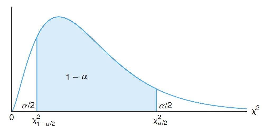
# Confidence Interval for 总体方差 的置信区间
If is the variance of a random sample of size from a , a confidence interval for is given by
大小为 的随机样本取自正态分布总体,样本方差为 ,则总体方差 的 置信区间可以表示为
where and are values of the chi-squared distribution with degrees of freedom, leaving areas of and , respectively, to the right.
其中, 和 表示自由度为 的, 和 区域的卡方分布的值
# Example 6
The following are the weights, in decagrams, of 10 packages of grass seed distributed by a certain company: 46.4, 46.1, 45.8, 47.0, 46.1, 45.9, 45.8, 46.9, 45.2, and 46.0.
某公司经销草种 10 包重量如下
Find a 95% confidence interval for the variance of the weights of all such packages of grass seed distributed by this company, assuming a normal population.
假设为正态总体,请计算该公司分发的所有此类草种包的重量的方差的 95% 置信区间。
weight <-c(46.4,46.1, 45.8, 47.0, 46.1, 45.9, 45.8, 46.9, 45.2,46.0) | |
n<- length(weight) | |
ssquare <- var(weight) | |
alpha <- 0.05 # 95% confidence interval | |
loBd <- (n-1)*ssquare/qchisq(1-alpha/2,n-1) | |
loBd |
[1] 0.1354167
upBd <- (n-1)*ssquare/qchisq(alpha/2,n-1) | |
upBd |
[1] 0.9539365
# In-class Exercise: Confidence Interval for
Please construct a 90% confidence interval for the variance of Sepal.Length of all records in iris data set.
请为数据集 iris 中 Sepal.Length 所有记录的方差构建一个 90% 的置信区间。
len <- iris$Sepal.Length | |
n <- length(len) | |
sampleVar <- var(len) | |
alpha <- 0.1 | |
loBd <- (n-1)*sampleVar/qchisq(1-alpha/2,n-1) | |
loBd |
[1] 0.5724186
upBd <- (n-1)*sampleVar/qchisq(alpha/2,n-1) | |
upBd |
[1] 0.8389097
# Estimating the Ratio of Two Variances 估计两个方差比
A point estimate of the ratio of two population variances is given by the ratio of the sample variances.
通过样本方差比为 ,对两个总体方差比 进行点估计。
Hence, the statistic is called an estimator of .
因此,统计量 被称为 的估计。
If and are the variances of normal populations, we can using the statistic
如果 和 是 正态群体的差异,我们可以使用统计量
to establish an interval estimate of .
来建立 的区间估计值。
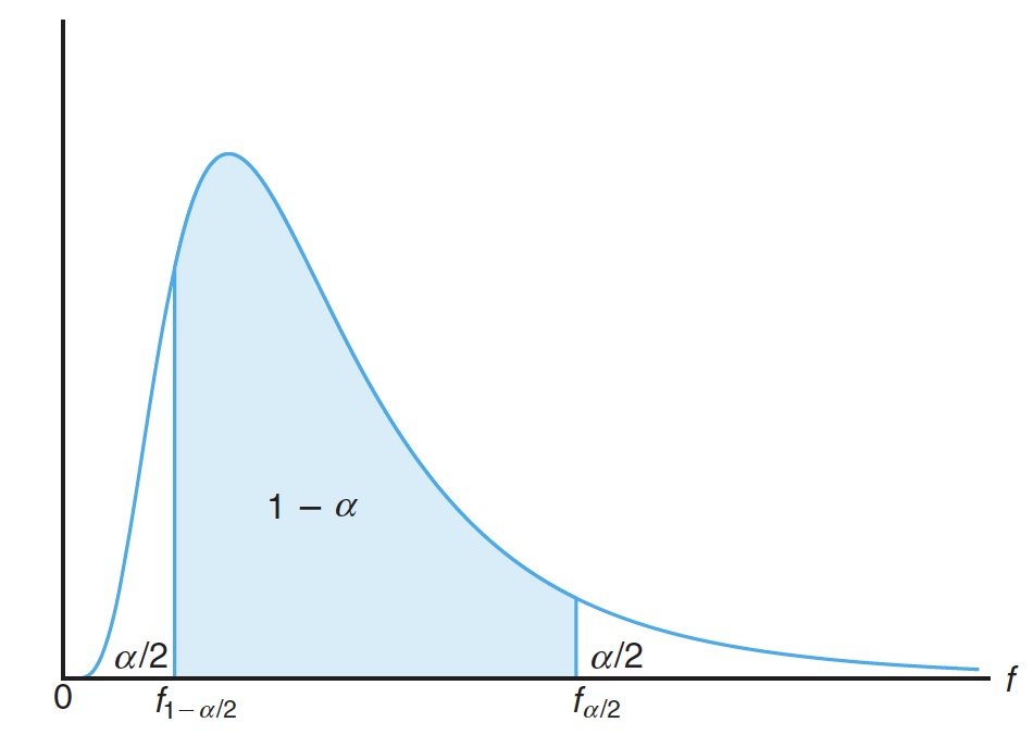
# Confidence Interval for 总体方差比 的置信区间
If and are the variances of a random sample of size and , respectively, from normal populations, then a confidence interval for is given by
两个随机样本取自正态总体,大小分别为 和 ,方差分别为 和 。总体方差比 的 置信区间可以表示为
where is an -value with and degrees of freedom, leaving an area of to the right, and is an -value with and degrees of freedom.
其中, 指取自自由度为 和 , 右侧区域的 值; 指自由度 和 的 值
# Example 7
A confidence interval for the difference in the mean orthophosphorus contents, measured in milligrams per liter, at two stations on the James River by assuming the normal population variance to be unequal.
河的两个站,假设正态总体的方差是不相等的,以每升毫克来测量两个站的平均磷含量的方差的置信区间。
Orthophosphorus was measured in milligrams per liter.
磷以每升毫克为单位测量。
Fifteen samples were collected from station 1, and 12 samples were obtained from station 2.
从 1 号站收集了 15 个样本,从 2 号站采集了 12 个样本。
The 15 samples from station 1 had an average orthophosphorus content of 3.84 milligrams per liter and a standard deviation of 3.07 milligrams per liter, while the 12 samples from station 2 had an average content of 1.49 milligrams per liter and a standard deviation of 0.80 milligram per liter.
1 号站的 15 个样品平均磷含量为每升 3.84 毫克,标准差为每升 3.07 毫克;2 号站的 12 个样品平均含量为每升 1.49 毫克,标准差为每升 0.80 毫克。
Justify this assumption by constructing 98% confidence intervals for and for , where and are the variances of the populations of
orthophosphorus contents at station 1 and station 2, respectively.
和 分别是 1 号站和 2 号站的磷含量总体方差,评估 和 的 98% 的置信区间
n1 <- 15 | |
n2 <- 12 | |
s1 <- 3.07 | |
s2 <- 0.80 | |
alpha <- 0.02 | |
loBd <- s1^2/s2^2/qf(1-alpha/2, n1-1, n2-1) | |
loBd |
[1] 3.430136
upBd <- s1^2/s2^2*qf(1-alpha/2, n2-1, n1-1) | |
upBd |
[1] 56.90341
Taking square roots of the confidence limits, we find that a 98% confidence interval for is
取置信区间的平方根,我们发现 98% 的置信区间是
Since this interval does not allow for the possibility of being equal to 1, we were correct in assuming that or .
由于此区间不存在 等于 1 的可能性,因此可以 或 假设是正确的
# In-class Exercise: Confidence Interval for 总体方差比 的置信区间
Please construct a 96% confidence interval for the ratio of variances of Sepal.Length between two species Setosa and Virginica in iris data set, i.e., , assume Sepal.Length of two species have approximately normal distributions.
请计算两个群体 Setosa 和 Virginica 的 Sepal.Length 的方差比的 96% 置信区间。假设这两个总体近似正态分布。
x1<-iris$Sepal.Length[iris$Species == 'virginica'] | |
x2<-iris$Sepal.Length[iris$Species == 'setosa'] | |
n1 <- length(x1) | |
sampleVar1 <- var(x1) | |
n2 <- length(x2) | |
sampleVar2 <- var(x2) | |
alpha <- 0.04 | |
loBd <- sampleVar1/sampleVar2/qf(1-alpha/2,n1-1, n2 -1) | |
loBd |
[1] 1.796658
upBd <- sampleVar1/sampleVar2*qf(1-alpha/2,n2-1, n1 -1) | |
upBd |
[1] 5.89452
# Conlusions
If we know the variances, we can use value to estimate or .
如果我们知道总体方差,我们可以使用 值 估计总体均值 或者 总体均值差 。If we don't know the variances, we should use value to estimate or and the distributions of the populations are approximately normal.
如果我们不知道总体方差,我们应该使用 值 估计总体均值 或者 总体均值差 ,并且总体的分布近似正态。To estimate for normal distributions, we need distribution; To estimate , we need -distribution.
估计正态分布的,需要 分布;估计,需要 分布。
# References
- Probability & Statistics for Engineers & Scientist, 9th Edition, Ronald E. Walpole, Raymond H. Myers, Sharon L. Myers, Keying Ye, Prentice Hall