# Objectives

• Understand Central Limit Theorem and when it can be used
  了解中心极限定理以及何时可以使用
• Know the sampling distribution of the sample mean, the difference between two means, the sample variance, and the ratio of two sample variances
  知道样本均值的抽样分布，两个均值的差值，样本方差，以及两个样本方差的比值
• Understand $t$ , $\chi^2$ , and $F$ distributions; in which situation, we should use these distributions
  理解 $t$，$\chi^2$，和 $F$ 分布；在哪种情况下，我们应该使用这些分布
• Know how to use q- and p- function to find the quantiles and probability of all these distributions
  知道如何使用 q- 和 p- 函数来找到所有这些分布的分位数和概率

# Review of Statistics 统计知识回顾

Population 群体

the entire group of individuals that we want information about.
我们想要了解的整个个群体体。

Sample 样本

a part of the population that we actually examine in order to gather information about the whole population.
我们实际检查的一部分人口，以收集有关整个人口的信息。

Inferential statistics 推论统计

use a fact about a sample to estimate the truth about the whole population.
使用关于样本的事实来估计关于整个总体的真相。

Sample Mean 样本均值

arithmetic average, denoted by $\bar{x}$
算术平均值，表示为 $\bar{x}$。

$$\bar{x} = \frac{x_1+\cdots+x_n}{n} = \frac{1}{n}\sum\limits_{i=1}^n x_i=\frac{1}{n}\sum x_i$$

Sample variance 样本方差

measure of variability, spread out, denoted by $s^2$
变异性的度量，分布，表示为 $s^2$。

$$s^2 = \frac{(x_1-\bar{x})^2+\cdots+(x_n-\bar{x})^2}{n-1} = \frac{\sum\limits_{i=1}^n (x_i-\bar{x})^2}{n-1}$$

# Distribution of Sample Mean 样本均值的分布

Central Limit Theorem CLT 中心极限定理

Let $\bar{X}$ be the mean of a random sample of size $n$ taken from a population with mean $\mu$ and finite variance $\sigma^2$, then the limiting of the limiting form of the distribution of
从均值为 $\mu$ 和有限方差为 $\sigma^2$ 的总群体中，取出大小为$n$ 的随机样本，该样本的平均值$\bar{X}$ 的分布极限形式的极限

$$Z = \frac{\bar{X} -\mu}{\sigma/\sqrt{n}}$$

as $n\rightarrow \infty$, is the standard normal distribution, i.e., $Z \sim \mathcal{N}(0,1)$.
当 $n\rightarrow \infty$ , 是呈标准正态分布，即 $Z \sim \mathcal{N}(0,1)$。

Remark 备注

• CLT can be summarized in one sentence:
  CLT 可以用一句话概括：
  When sample size $n$ is large ($n>30$), approximately,
  当样本量 $n$ 很大（$n>30$），则其均值大约为，

  $$\bar{X}\sim \mathcal{N}(\mu, \sigma^2/n)$$

• The mean and standard deviation of sample mean from a population with mean $\mu$ and standard deviation $\sigma$ are always:
  总体均值为 $\mu$ 、标准差为 $\sigma$ ，其样本均值的均值和标准差

  $$\mu_{\bar{X}} = \mu, \qquad \sigma_{\bar{X}} = \frac{\sigma}{\sqrt{n}}$$

  regardless of population distribution and sample size $n$.
  无论群体分布和样本大小 $n$ 如何。

• The Central Limit Theorem simply provides us the shape of the distribution of sample mean when the sample size is large.
  中心极限定理只是为我们提供了样本量较大时，样本均值分布的形态。

# Example 1 pnorm()

When a batch of a certain chemical product is prepared, the amount of a particular impurity in the batch is a random variable with mean value 4.0 g and standard deviation 1.5 g. If 50 batches are independently prepared, what is the (approximate) probability that the sample average amount of impurity $\bar{X}$ is between 3.5 and 3.8 g?
某化工产品的批次制备时，批次中特定杂质的含量为随机变量，均值为 4.0 g，标准差为 1.5 g。如果独立制备 50 个批次，样品平均杂质含量$\bar{X}$ 介于 3.5 和 3.8 克之间的（近似）概率是多少？

nsize<- 50 # Sample Size

a <- 3.5  

b <- 3.8

mu <- 4 # Mean of Sample Mean

standardDev <- 1.5/sqrt(nsize) # Sd of Sample Mean

p <- pnorm(b, mean = mu, sd = standardDev)- pnorm(a, mean = mu, sd = standardDev)

p

[1] 0.1636782

# In-class Exercise: Sample Mean Distribution 样本均值分布

The amount of time that a drive-through bank teller spends on a customer is a random variable with a mean $\mu = 3.2$ minutes and a standard deviation $\sigma = 1.6$ minutes. If a random sample of 64 customers is observed, find the probability that their mean time at the teller’s window is
银行柜员在客户身上花费的时间是一个随机变量，其均值 $\mu = 3.2$ 分钟、标准差 $\sigma = 1.6$ 分钟。如果一个随机样本观察 64 位顾客，求他们在柜员窗口的平均时间为

1. at most 2.7 minutes;
   最多 2.7 分钟；

   	# X <= 2.7
   	samplesize<-64
   	mu <- 3.2
   	sigma<- 1.6/sqrt(samplesize)
   	p1<-pnorm(2.7,mean = mu, sd = sigma)
   	p1

   [1] 0.006209665
   

2. more than 3.5 minutes;
   超过 3.5 分钟；

   	# X > 3.5
   	p2<-1-pnorm(3.5,mean = mu, sd = sigma)
   	p2

   [1] 0.0668072
   

3. at least 3.2 minutes but less than 3.4 minutes.
   至少 3.2 分钟但少于 3.4 分钟。

   	# 3.2<= X < 3.4
   	p3<-pnorm(3.4,mean = mu, sd = sigma)-pnorm(3.2,mean = mu, sd = sigma)
   	p3

   [1] 0.3413447
   

# Sampling Distribution of the Difference between Two Means 两个均值之间差异的抽样分布

# The normal distribution 正态分布

A scientist or engineer may be interested in a comparative experiment in which two manufacturing methods, 1 and 2, are to be compared.
科学家或工程师可能对比较实验感兴趣，其中要比较两种制造方法 1 和 2。

The basis for the comparison is the difference in the population means.
比较的基础是总体均值之间的差异。

Suppose that we have two populations, the first with mean $\mu_1$ and variance $\sigma_1^2$, and the second with mean $\mu_2$ and variance $\sigma_2^2$.
假设我们有两个总体，第一个具有均值 $\mu_1$ 和方差 $\sigma_1^2$，第二个具有均值 $\mu_2$ 和方差 $\sigma_2^2$.

Theorem 定理

If independent samples of size $n_1$ and $n_2$ are drawn at random from two populations, discrete or continuous, with means $\mu_1$ and $\mu_2$ and variances $\sigma_1^2$ and $\sigma_2^2$, respectively, then the sampling distribution of the differences of means, $\bar{X}_1-\bar{X}_2$, is approximately normally distributed with mean and variance given by
如果从均值分别为 $\mu_1$ 和 $\mu_2$ 、方差分别为 $\sigma_1^2$ 和 $\sigma_2^2$ 的两个离散或连续的群体中，随机抽取大小为 $n_1$ 和 $n_2$ 的独立样本，则两个样本的均值差$\bar{X}_1-\bar{X}_2$ 的抽样分布，近似正态分布，均值和方差由下式给出

$$\mu_{\bar{X}_1-\bar{X}_2} = \mu_1-\mu_2, \qquad \sigma_{\bar{X}_1-\bar{X}_2}^2 = \frac{\sigma^2_1}{n_1} + \frac{\sigma_2^2}{n_2}$$

Hence,

$$Z = \frac{\left(\bar{X}_1-\bar{X}_2\right)-(\mu_1-\mu_2)}{\sqrt{\sigma^2_1/n_1 + \sigma_2^2/n_2}} \sim \mathcal{N}(0,1)$$

Remark 备注

If both $n_1$ and $n_2$ are greater than or equal to 30, the normal approximation for the distribution of $\bar{X}_1-\bar{X}_2$ is very good when the distributions are not too far away from normal.
如果样本量 $n_1$ 和 $n_2$ 均大于或等于 30，均值差 $\bar{X}_1-\bar{X}_2$ 分布的正态近似值非常好，分布接近正态分布。

# Example 2

The television picture tubes of manufacturer $A$ have a mean lifetime of 6.5 years and a standard deviation of 0.9 year, while those of manufacturer $B$ have a mean lifetime of 6.0 years and a standard deviation of 0.8 year.
制造商 $A$ 的电视显像管 平均寿命为 6.5 年，标准差为 0.9 年，而制造商 $B$ 的是平均寿命为 6.0 年，标准差为 0.8 年。

What is the probability that a random sample of 36 tubes from manufacturer $A$ will have a mean lifetime that is at least 1 year more than the mean lifetime of a sample of 49 tubes from manufacturer $B$?
制造商 $A$ 的 36 个管子的随机样本的平均寿命，比制造商 $B$ 的 49 个管子样本的平均寿命至少多 1 年的概率是多少？

# We can solve it in two ways

# Method I:

n1<- 36 # Sample Size of population 1

n2<- 49 # Sample size of population 2

mu1<- 6.5 # Mean of population 1

mu2<- 6.0 # Mean of population 2

sigma1<- 0.9 # Std of population 1

sigma2<- 0.8 # Std of population 2

value <- 1.0

p1<- 1- pnorm(value, mean = mu1-mu2, sd =sqrt(sigma1^2/n1 + sigma2^2/n2))

p1

[1] 0.004007479

# Method II:

zvalue <- (value - (mu1-mu2))/sqrt(sigma1^2/n1 + sigma2^2/n2) 

p2<- 1- pnorm(zvalue)

p2

[1] 0.004007479

# In-class Exercise: Difference between Two Means 两个均值的差别

Two different box-filling machines are used to fill cereal boxes on an assembly line.
两台不同的装盒机用于在装配线上装满谷物盒。

The critical measurement influenced by these machines is the weight of the product in the boxes.
受这些机器影响的关键测量是箱子中产品的重量。

Engineers are quite certain that the variance of the weight of product is $\sigma^2 = 1$ ounce.
工程师非常确定产品重量的方差是 $\sigma^2 = 1$ 盎司。

Experiments are conducted using both machines with sample sizes of 36 each.
使用两台机器进行实验，每台机器的样本量为 36。

The sample averages for machines $A$ and $B$ are $\bar{x}_A = 4.5$ ounces and $\bar{x}_B = 4.7$ ounces.
机器样本 $A$ 和$B$ 的平均值分别是$\bar{x}_A = 4.5$ 盎司和 $\bar{x}_B = 4.7$ 盎司。

Engineers are surprised that the two sample averages for the filling machines are so different.
工程师们惊讶于灌装机的两个样本平均值如此不同。

(a) Use the Central Limit Theorem to determine
使用中心极限定理来确定

$$P(\bar{X}_B-\bar{X}_A \ge 0.2)$$

under the condition that $\mu_A = \mu_B$.
在 $\mu_A = \mu_B$ 这样的条件下。

(b) Do the aforementioned experiments seem to, in any way, strongly support a conjecture that the population means for the two machines are different? Explain using your answer in a.
上述实验是否似乎以任何方式强烈支持两台机器的总体均值不同的猜想？使用你在 a 中的答案进行解释。

n <- 36 # Sample Size of population 1 & 2

sigma<- 1 # Std of population 1 & 2

value <- 0.2

p1<- 1 - pnorm(value, mean =0, sd =sqrt(2*sigma^2/n))

p1

[1] 0.198072

Question: If we have no idea about the population variance, what can we do?
如果我们不知道总体方差，我们能做什么？

# The $t$ Distribution $t$ 分布

Let $X_1, X_2,...,X_n$ is a random sample from a normal distribution $\mathcal{N}(\mu, \sigma^2)$. Let
从一个正态分布中取出一个随机样本，让

$$\bar{X} = \frac{1}{n}\sum_{i=1}^n X_i, \qquad S^2 = \frac{1}{n-1}\sum_{i=1}^n (X_i-\bar{X})^2$$

Then the random variable

$$T = \frac{\bar{X}-\mu}{S/\sqrt{n}}$$

has the $t$ distribution with $v = n-1$ degrees of freedom, $t_{n-1}$.
随机变量呈$t$ 分布，其自由度为 $v = n-1$，t_

Remark

The $t$-distribution can still be used even if the population distribution is not normal, as long as
即使总体分布不符合正态分布，$t$ 分布仍然可以使用，只要

• the sample size $n$ is large.
  样本量$n$ 很大
• the population distribution is not too-skewed.
  总体分布并不太偏。

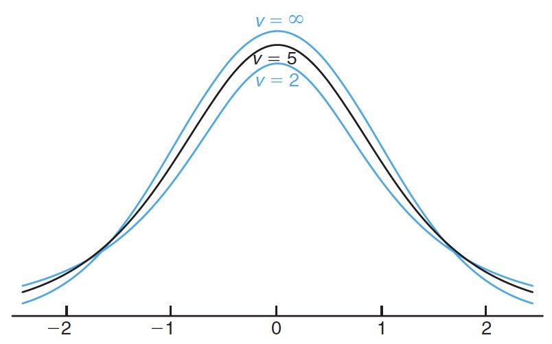
The following is the graph of the pdf of $t$ distribution with different degrees of freedom. As the degrees of freedom $v$ gets large, the pdf gets closer to normal curve.
以下是不同自由度的$t$ 分布的 pdf 图表。自由度 $v$ 变大，pdf 越来越接近正态曲线。

# Example 3 qt

A chemical engineer claims that the population mean yield of a certain batch process is 500 grams per milliliter of raw material.
一位化学工程师声称某个批处理过程的总体平均产量是每毫升原材料 500 克。

To check this claim he samples 25 batches each month.
为了核实这一说法，他每个月抽取 25 批样品。

If the computed $t-$value falls between $-t_{0.05}$ and $t_{0.05},$ he is satisfied with this claim.
如果计算出的$t$ 值介于 $-t_{0.05}$ 和 $t_{0.05},$ 他对这一说法感到满意。

What conclusion should he draw from a sample that has a mean $\bar{x} = 518$ grams per milliliter and a sample standard deviation $s = 40$ grams? Assume the distribution of yields to be approximately normal.
他应该从均值$\bar{x} = 518$ g/ml 和标准差 $s = 40$ g 的样本中得出什么结论？假设产量分布近似正态。

# To get t_{0.05} with v = 24

alpha <- 0.05

v <- 24

tvalue <- qt(1 - alpha, v)

tvalue

[1] 1.710882

# Or we can get -t_{0.05} with v = 24 first

tnegvalue <- qt(alpha, v)

tnegvalue

[1] -1.710882

# In-class Exercise: $t$ Distribution

A manufacturing firm claims that the batteries used in their electronic games will last an average of 30 hours.
一家制造公司声称，他们电子游戏中使用的电池平均可以使用 30 小时。

To maintain this average, 16 batteries are tested each month.
为了保持这一平均值，每月测试 16 节电池。

If the computed t-value falls between $-t_{0.025}$ and $t_{0.025}$, the firm is satisfied with its claim.
如果计算出的 t 值介于 $-t_{0.025}$ 和 $t_{0.025}$，公司对其索赔表示满意。

What conclusion should the firm draw from a sample that has a mean of $\bar{x}= 27.5$ hours and a standard deviation of $s = 5$ hours? Assume the distribution of battery lives to be approximately normal.
公司应该从具有均值$\bar{x}= 27.5$ 小时数和标准差 $s = 5$ 小时的样本中得出什么结论？假设电池寿命分布近似正态。

n <- 16

s <- 5

xbar <- 27.5

mu <- 30

tstats <- (xbar - mu)/(s/sqrt(n))

tstats

[1] -2

# To get t_{0.025} with v = 15

alpha <- 0.05

v <- 15

tvalue <- qt(1 - alpha/2, v)

tvalue

[1] 2.13145

# Or we can get -t_{0.052} with v = 15 first

tnegvalue <- qt(alpha/2, v)

tnegvalue

[1] -2.13145

# Sampling Distribution of Sample Variance 样本方差的抽样分布

# The Chi-Squared Distribution 卡方分布

Chi-squared distribution is usually used when we seek some conclusion on variance of a population.
当我们寻求关于总体方差的一些结论时，通常使用卡方分布。

If $S^2$ is the variance of a random sample of size $n$ taken from a normal population having the variance $\sigma^2$, then the statistic
如果大小为 $n$ 的随机样本的方差为 $S^2$ ，该样本取自方差为 $\sigma^2$ 的正态总体，那么统计量

$$\chi^2 = \frac{(n-1)S^2}{\sigma^2} = \sum_{i=1}^n \frac{(X_i-\bar{X})^2}{\sigma^2}$$

has a chi-squared distribution with $v = n - 1$ degrees of freedom.
呈自由程度为 $v = n - 1$ 的卡方分布。

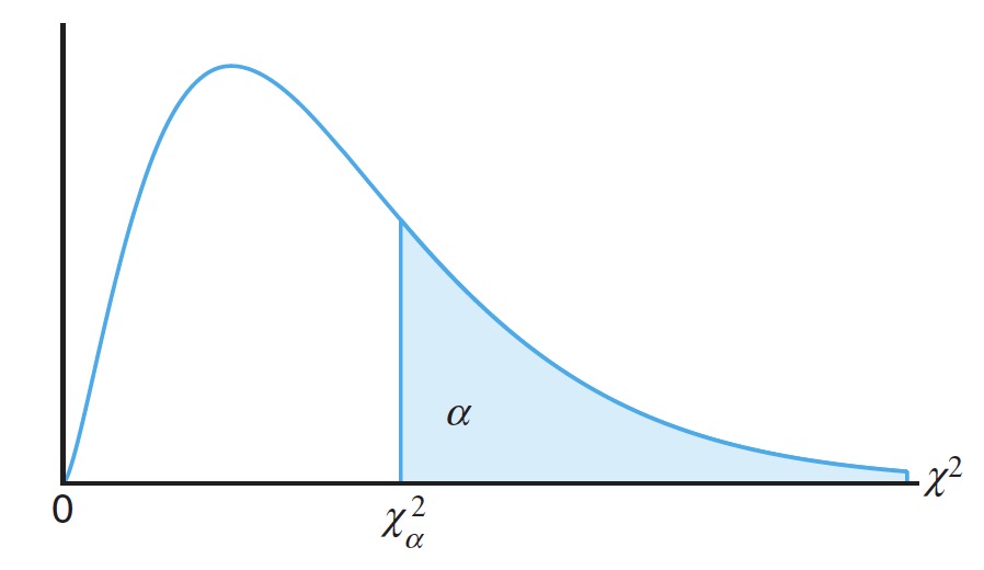
The probability that a random sample produces a $\chi^2$ value greater than some specified value is equal to the area under the curve to the right of this value.
随机样本产生一个 $\chi^2$ 值大于某个指定值的概率，等于该值右侧曲线下的面积。

It is customary to let $\chi^2_\alpha$ represent the $\chi^2$ value above which we find an area of $\alpha$. This is illustrated by the shaded region in the following figure.
习惯上让 $\chi^2_\alpha$ 代表我们在该高于 $\alpha$ 区域找到的 $\chi^2$ 值。下图中的阴影区域说明了这一点。

# Example 4 qchisq

A manufacturer of car batteries guarantees that the batteries will last , on average 3 years with a sandard deviation of 1 year.
汽车电池制造商保证电池使用寿命平均为 3 年，标准偏差为 1 年。

If five of these batteries have lifetimes of $1.9, 2.4, 3.0, 3.5,$ and $4.2$ years, should the manufacturer still be convinced that the batteries have a standard deviation of 1 year?
如果其中五个电池的使用寿命为 1.9 , 2.4 , 3.0 , 3.5 和 4.2 年，制造商是否应该仍然相信电池有 1 年的标准偏差？

Assume that the battery lifetime follows a normal distribution. Let's consider $\alpha = 0.05$.
假设电池寿命服从正态分布，并考虑 $\alpha = 0.05$。

alpha <- 0.05

v <- 4

# Get chisq_{0.05/2} when v = 4 

chiLeftValue <- qchisq(alpha/2, v)

chiLeftValue

[1] 0.4844186

# Get chisq_{ 1 - 0.05/2} when v = 4

chiRightValue<- qchisq(1-alpha/2, v)

chiRightValue

[1] 11.14329

# In-class Exercise: $\chi^2$ Distribution

1. For a chi-squared distribution, find
   对于卡方分布，找到

   • $\chi^2_{0.025}$ when $v = 15$;
   • $\chi^2_{0.01}$ when $v = 7$;
   • $\chi^2_{0.05}$ when $v = 24$;

   qchisq(1-0.025,15)

   [1] 27.48839
   

   qchisq(1-0.01,7)

   [1] 18.47531
   

   qchisq(1-0.05,24)

   [1] 36.41503
   

2. The scores on a placement test given to college freshmen for the past five years are approximatedly normally distributed with a mean $\mu= 74$ and a variance $\sigma^2 =8$.
   过去五年大学新生的分班考试分数近似一个均值$\mu= 74$ 和方差 $\sigma^2 =8$ 的正态分布。
   would you still consider $\sigma^2 = 8$ to be a valid value of the variance if a random sample of 20 students who take the placement test this year obtain a value of $s^2 = 20$?
   如果今年参加分级考试的 20 名学生的随机样本有 $s^2 = 20$，是否仍将 $\sigma^2 = 8$ 视为方差的有效值？

   	ssquared <- 20
   	sigmasquared <- 8
   	n <- 20
   	chisqstats <- (n-1)*ssquared/sigmasquared
   	chisqstats

   [1] 47.5
   

   	alpha <- 0.05
   	loBound <- qchisq(alpha/2,n-1)
   	loBound

   [1] 8.906516
   

   	upBound <- qchisq(1-alpha/2,n-1)
   	upBound

   [1] 32.85233
   

# The $F$ Distribution $F$ 分布

Suppose that we have a random sample of $m$ observations from the normal population $\mathcal{N}(\mu_1,\sigma_1^2)$ and an independent random sample of $n$ observations from a second normal population $\mathcal{N}(\mu_2,\sigma_2^2)$.
假设我们有一个随机样本 $m$ 来自正态总体 $\mathcal{N}(\mu_1,\sigma_1^2)$ ，以及一个独立的随机样本 $n$ 来自第二个正态总体 $\mathcal{N}(\mu_2,\sigma_2^2)$ 。

Then,

$$F_{m-1,n-1} = \frac{S_1^2/\sigma_1^2}{S_2^2/\sigma_2^2},$$

follows an $F$ distribution with $v_1 = m-1$ and $v_2 = n-1$, where $S_1$, $S_2$ and $\sigma_1$, $\sigma_2$ are sample and population standard deviations of sample 1 and sample 2, respectively.
分别遵循自由度为 $v_1 = m-1$ 和 $v_2 = n-1$ 的 $F$ 分布，其中 $S_1$、$S_2$ 和 $\sigma_1$、$\sigma_2$ 分别是样本 1 和样本 2 的样本标准差和总体标准差。

This $F$ statistic can be used to compare variances from two independent groups.
此 $F$ 统计量可用于比较来自两个独立组的差异。

Here are some density curves of $F$ distribution with different degrees of freedoms:
这是不同自由度的 $F$ 分布的密度曲线：

$$f_{1-\alpha}(v_1,v_2) = \frac{1}{f_\alpha(v_2,v_1)}$$

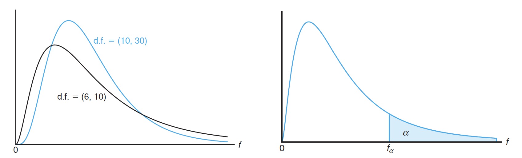
The $F-$distribution finds enormous application in comparing sample variances.
$F$ 分布在比较样本方差方面有着巨大的应用。

Applications of the $F-$distribution are found in problems involving two or more samples.
$F$ 分布多应用在涉及两个或更多样本的问题中。

# Example 5 qf

Pull-strength tests on 10 soldered leads for a semiconductor device yield the following results, in pounds of force required to rupture the bond: 19.8 12.7 13.2 16.9 10.6 18.8 11.1 14.3 17.0 12.5
对半导体器件的 10 根焊接引线进行拉力测试，得出以下结果，破坏键合所需的力以磅为单位：19.8 12.7 13.2 16.9 10.6 18.8 11.1 14.3 17.0 12.5

Another set of 8 leads was tested after encapsulation to determine whether the pull strength had been increased by encapsulation of the device, with the following results: 24.9 22.8 23.6 22.1 20.4 21.6 21.8 22.5
封装后测试另一组 8 根引线，以确定器件的封装是否增加了拉力，结果如下：24.9 22.8 23.6 22.1 20.4 21.6 21.8 22.5

Comment on the evidence available concerning equality
of the two population variances.
评论关于两个总体方差相等的现有证据。

sample1 <- c(19.8,12.7,13.2,16.9,10.6,18.8,11.1 ,14.3,17.0,12.5)

s1<- sd(sample1)

sample2 <- c(24.9,22.8,23.6,22.1,20.4,21.6,21.8 ,22.5)

s2<- sd(sample2)

fvalue<- s1^2/s2^2 # as sigma1 = sigma2

fvalue

[1] 5.657436

alpha <- 0.01

m <- 10

n <- 8

f1q <- qf(alpha/2, m-1,n-1)

f1q

[1] 0.1452452

f2q <- qf(1-alpha/2,m-1,n-1)

f2q

[1] 8.513823

# Conclusion

1. Distribution of sample mean/difference between two means with known variance when sample size is large enough is normal distribution.
   当样本大小足够大时，两个已知方差的样本均值 / 差值分布是正态分布的。

2. With unknown variance, the instance comes from the normal distribution, then the sample mean follows a $t$ distribution
   方差未知，实例来自正态分布，则样本均值遵循 $t$ 分布

3. $\chi^2$ distribution is used for sample variance.
   $\chi^2$ 分布用于样本方差。

4. $F$ distribution is used for the ratio of two variances.
   $F$ 分布用于两个方差的比率。

# References

1. Probability & Statistics for Engineers & Scientist, 9th Edition, Ronald E. Walpole, Raymond H. Myers, Sharon L. Myers, Keying Ye, Prentice Hall