# Objective

Confidence Interval V.S. Prediction Interval
置信区间与预测区间
Qualitative Predictors
定性预测因子
Extension of the Linear Models
线性模型的扩展

# Goodness-of-Fit Test 拟合优度检验

# Overview

What is Goodness-of-Fit Test?

It is a test to determine if a population has a specified theoretical distribution.
这是一个检验，用来确定一个总体是否具有特定的理论分布。

The test is based on how good a fit we have between the frequency of occurrence of observations in an observed sample and the expected frequencies obtained from the hypothesized distribution.
该检验基于观测样本中观测值出现的频率与从假设分布中获得的预期频率之间的良好拟合程度。

# Illustrating Example 例子说明

we consider the tossing of a die.
我们考虑掷骰子。

We hypothesize that the die is honest, which is equivalent to testing the hypothesis that the distribution of outcomes is the discrete uniform distribution
我们假设骰子是诚实的，这相当于检验假设结果的分布是离散均匀分布

$f(x) = \frac{1}{6}, \qquad x = 1,2, \ldots, 6.$

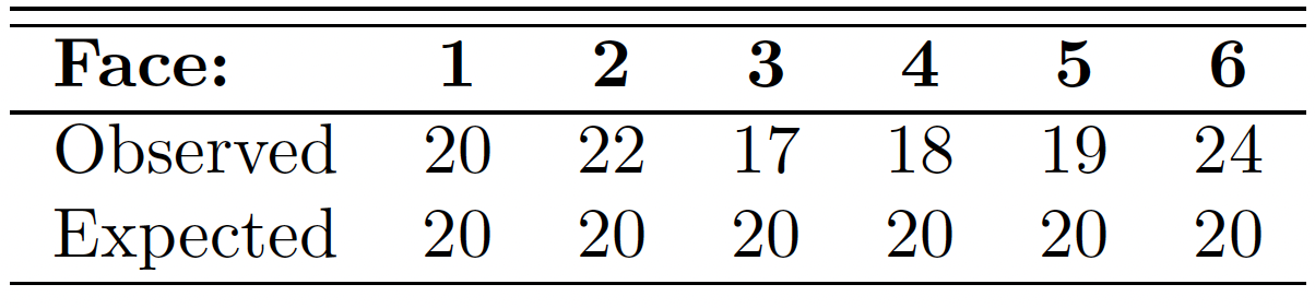
Suppose that the die is tossed 120 times and each outcome is recorded.
假设掷骰子 120 次，每个结果都被记录下来。

Theoretically, if the die is balanced, we would expect each face to occur 20 times.
理论上，如果骰子是平衡的，我们期望每个面出现 20 次。

The results are given in the following table.
结果如下表所示。

A goodness-of-fit test between observed and expected frequencies is based on the quantity
观察到的频率和期望频率之间的拟合优度测试是基于数量的

$\chi^2 = \sum_{i=1}^k\frac{(o_i-e_i)^2}{e_i},$

where $\chi^2$ is a value of a random variable whose sampling distribution is approximated very closely by the chi-squared distribution with $v = k - 1$ degrees of freedom.
其中 $\chi^2$ 是一个随机变量的值，该随机变量的抽样分布非常接近于具有 $v = k - 1$ 自由度的卡方分布。

The symbols $o_i$ and $e_i$ represent the observed and expected frequencies, respectively, for the ith cell.
符号 $o_i$ 和 $e_i$ 分别表示第 i 个单元的观测频率和期望频率。

If the observed frequencies are close to the corresponding expected frequencies, the $\chi^2$ -value will be small, indicating a good fit.
如果观测到的频率接近于相应的预期频率， $\chi^2$ 的值将很小，表明一个良好的拟合。

If the observed frequencies differ considerably from the expected frequencies, the $\chi^2$ -value will be large and the fit is poor.
如果观测到的频率与预期的频率有很大的差异， $\chi^2$ 的值将会很大，拟合很差。

A good fit leads to the acceptance of $H_0$ , whereas a poor fit leads to its rejection.
良好的拟合导致 $H_0$ 被接受，而糟糕的拟合导致 $H_0$ 被拒绝。

The critical region will, therefore, fall in the right tail of the chi-squared distribution.
因此，临界区域将落在卡方分布的右尾。

For a level of significance equal to $\alpha$ , we find the critical value $\chi^2_\alpha$ , and then $\chi^2 > \chi^2_\alpha$ constitutes the critical region.
对于等于 $\alpha$ 的显著性水平，我们找到临界值 $\chi^2_\alpha$ ，然后 $\chi^2 > \chi^2_\alpha$ 构成临界区域。

The decision criterion described here should not be used unless each of the expected frequencies is at least equal to 5.
除非每个预期频率至少等于 5，否则不应使用此处描述的判定标准。

$\chi^2 = \frac{(20-20)^2}{20} + \frac{(22-20)^2}{20} + \frac{(17-20)^2}{20} \\ \frac{(18-20)^2}{20} + \frac{(19-20)^2}{20} + \frac{(24-20)^2}{20} = 1.7.$

	alpha <- 0.05
	qchisq(1-alpha,5)

[1] 11.0705

We can find $\chi^2 < \chi^2_\alpha$ , we fail to reject $H_0$ .
我们可以找到 $\chi^2 < \chi^2_\alpha$ ，因此无法拒绝 $H_0$ 。

We conclude that there is insufficient evidence that the die is not balanced.
我们的结论是，没有足够的证据表明模具不平衡。

Can we use test in r to solve it? Yes.

	#the observation
	obs <- c(20,22, 17, 18, 19,24)
	#Here we provide the theoretical distribution via p value
	chiTest<-chisq.test(obs, p = rep(1/6,6))
	chiTest

    Chi-squared test for given probabilities

data:  obs
X-squared = 1.7, df = 5, p-value = 0.8889

We can find the $\chi^2$ statistic is exactly the same as what we got from the formula.
我们可以发现 $\chi^2$ 统计数据与我们从公式中得到的数据完全相同。

As p-value is much larger than $\alpha = 0.05$ , we should not reject $H_0$ .
由于 p 值远大于 $\alpha=0.05$ ，我们不应拒绝 $H_0$ 。

Can we use prop.test ?

prop.test(x = obs, n= rep(120,6))

    6-sample test for equality of proportions without continuity
    correction

data:  obs out of rep(120, 6)
X-squared = 2.04, df = 5, p-value = 0.8436
alternative hypothesis: two.sided
sample estimates:
   prop 1    prop 2    prop 3    prop 4    prop 5    prop 6 
0.1666667 0.1833333 0.1416667 0.1500000 0.1583333 0.2000000

Note: When the sample size is greater than 2, the continuity correction is never used. Why?
当样本大小大于 2 时，永远不会使用连续性校正。为什么？

The continuous chi-squared distribution seems to approximate the discrete sampling distribution of $\chi^2$ very well, provided that the number of degrees of freedom is greater than 1.
如果自由度数大于 1，则连续卡方分布似乎非常接近离散采样分布 $\chi^2$

In a 2 $\times$ 2 contingency table, where we have only 1 degree of
freedom, a correction called Yates’ correction for continuity is applied.
在 2 $\times$ 2 列联表中，我们只有 1 个自由度，应用耶茨连续性校正方法修正。

The corrected formula then becomes
修正后的公式就变成了

$\chi^2(corrected) = \sum_{i = 1}\frac{(|o_i-e_i|-0.5)^2}{e_i}.$

Contingency table 列联表: is a table with observed frequencies.
是一个有观测频率的表。
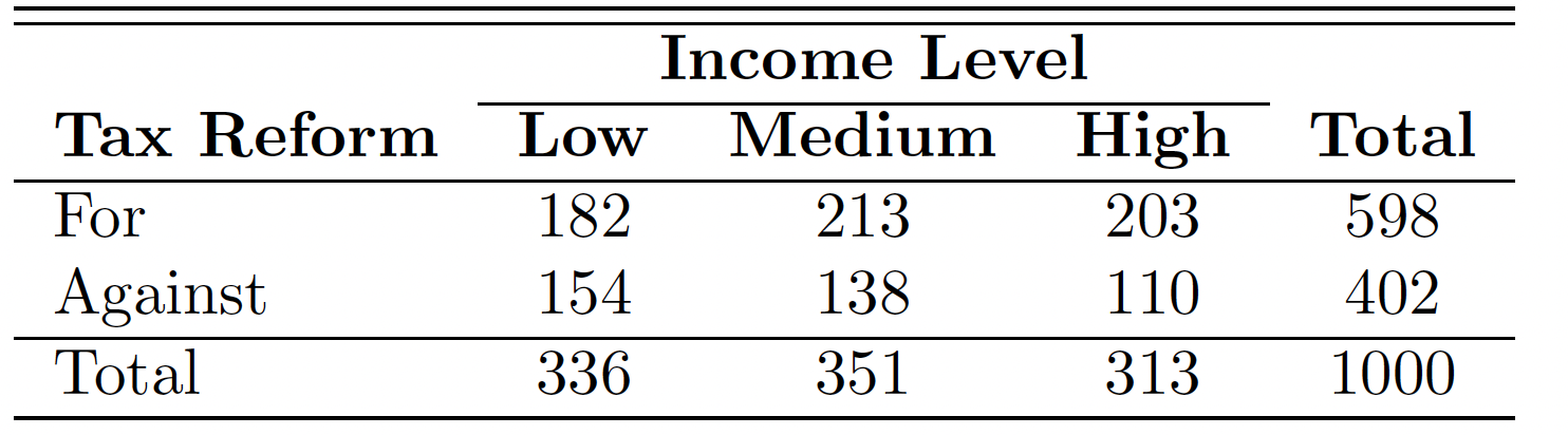
The following is $2 \times 3$ contingency table.
下面是 $2 \times 3$ 关联表。

How to use chisq.test ?

	# Manually enter the data
	taxreform <- rbind(c(182,213,203), c(154,138,110))
	dimnames(taxreform) <- list(
	reform = c("For", "Against"),
	IncomeLevel = c("Low","Medium", "High"))
	# display the data
	taxreform

         IncomeLevel
reform    Low Medium High
  For     182    213  203
  Against 154    138  110

	# display the proportion
	prop.table(taxreform)

         IncomeLevel
reform      Low Medium  High
  For     0.182  0.213 0.203
  Against 0.154  0.138 0.110

	# chi-square test
	chisq.test(taxreform)

    Pearson's Chi-squared test

data:  taxreform
X-squared = 7.8782, df = 2, p-value = 0.01947

Why degree freedom is 2? Actually
为什么自由度是 2？实际上

$v = (r-1)(c-1),$

where $r$ is # of rows and $c$ is # of columns.
其中 $r$ 是行号， $c$ 是列号。

We can't use prop.test here.
这里不能用 prop.test

# In-Class Exercise

There are 848 observations in before2013 dataset and 49 of those with Type.of.Breach == "Hacking/IT Incident" .
在 before2013 数据集中有 848 个观测值，其中 49 个带有 Type.of.Breach == "Hacking/IT Incident" 。

For after2013 dataset, there are 303 observations and 28 of those with Type.of.Breach == "Hacking/IT Incident" .
对于 after2013 数据集，有 303 个观测值，其中有 28 个带有 Type.of.Breach == "Hacking/IT Incident" 。

Can you construct a contingency table and test with chisq.test ? What about prop.test ?
你能构造一个列联表并使用 chisq.test 进行测试吗？ prop.test 呢？

	breachTable <-rbind(c(49,799),c(28,275))
	dimnames(breachTable) <- list(
	year = c("before2013", "after2013"),
	breachType = c("Hacking/IT Incident","Others"))
	# display the data
	breachTable

##             breachType
## year         Hacking/IT Incident Others
##   before2013                  49    799
##   after2013                   28    275

	# display the proportion
	prop.table(breachTable)

##             breachType
## year         Hacking/IT Incident    Others
##   before2013          0.04257168 0.6941790
##   after2013           0.02432667 0.2389227

	# chi-square test
	chisq.test(breachTable)

## 
##  Pearson's Chi-squared test with Yates' continuity correction
## 
## data:  breachTable
## X-squared = 3.751, df = 1, p-value = 0.05278

	# prop test
	prop.test(breachTable)

## 
##  2-sample test for equality of proportions with continuity correction
## 
## data:  breachTable
## X-squared = 3.751, df = 1, p-value = 0.05278
## alternative hypothesis: two.sided
## 95 percent confidence interval:
##  -0.073059117  0.003806673
## sample estimates:
##     prop 1     prop 2 
## 0.05778302 0.09240924

# Confidence vs. prediction intervals

# Revisit `Auto` Example

	require(ISLR)
	data(Auto)

Auto data set, regression on Y=mpg vs. X=horsepower .
Auto 数据集，回归 Y=mpg vs. X=horsepower 。

fitLm <- lm(mpg ~ horsepower, data=Auto)

What is the predicted mpg associated with a horsepower of $98$ ? What are the associated 95% confidence and prediction intervals?
与 horsepower 为 $98$ 的相关的预测 mpg 是多少？相关的 95% 置信区间和预测区间是什么？

	new <- data.frame(horsepower = 98)
	predict(fitLm, new) # predicted mpg

       1 
24.46708

predict(fitLm, new, interval="confidence") # conf interval

       fit      lwr      upr
1 24.46708 23.97308 24.96108

predict(fitLm, new, interval="prediction") # pred interval

       fit     lwr      upr
1 24.46708 14.8094 34.12476

Three sorts of uncertainty associated with the prediction of $Y$ based on $X_1,\dots,X_p$ :
基于 $X_1$ 、 $\dots$ 、 $X_p$ ，预测 $Y$ 的三种不确定性:

$\hat\beta_i\approx\beta_i$ $\hat{β}_{i} \approx β_{i}$ : least squares plane is an estimate for the true regression plane.
最小二乘平面是对真实回归平面的估计。
- reducible error
  可约误差
assuming a linear model for $f(X)$ $f (X)$ is usually an approximation of reality
假设 $f(X)$ $f (X)$ 的线性模型通常是现实的近似值
- model bias [potential reducible error?]
  模型偏差【潜在的可减少误差？】
- to operate here, we ignore this discrepancy
  为了在这里操作，我们忽略这个差异
even if we knew true $\beta_i$ $β_{i}$ , still no perfect knowledge of $Y$ $Y$ because of random error $\epsilon$ $ϵ$
即使我们知道 $\beta_i$ $β_{i}$ 为真，由于随机错误 $\epsilon$ $ϵ$ ，仍然不完全知道 $Y$ $Y$
- irreducible error
  不可约误差
- how much will $Y$ vary from $\hat Y$ ?
  $Y$ 和 $\hat Y$ 有多少区别？
- we use prediction intervals. Always wider than confidence intervals.
  我们使用预测区间。始终大于置信区间。

# `Advertising` confidence 可信度

Confidence interval 置信区间: Quantify the uncertainty surrounding the average sales over a large number of cities.
量化大量城市平均销售额的不确定性。

For example:

given that $100,000 is spent on TV advertising and
10 万美元用于电视广告
$20,000 is spent on radio advertising in each city,
广播广告花费 2 万美元
the 95% confidence interval is [10,985, 11,528] .
95% 的置信区间
We interpret this to mean that 95% of intervals of this form will contain the true value of $f(X)$ .
我们对此的解释是，此形式的 95% 的区间将包含 $f(X)$ 的真实值。

# `Advertising` prediction 预测

Prediction interval 预测区间: Can be used to quantify the uncertainty surrounding sales for a particular city.
可用于量化特定城市销售的不确定性。

Given that $100,000 is spent on TV advertising and
10 万美元用于电视广告和
$20,000 is spent on radio advertising in that city
2 万美元做广播广告
the 95% prediction interval is [7,930, 14,580] .
95% 的预测区间
We interpret this to mean that 95% of intervals of this form will contain the true value of $Y$ for this city.
我们对此的解释是，此形式的 95% 的区间将包含该城市 $Y$ 的真实值

Note that both intervals are centered at 11,256, but that the prediction interval is substantially wider than the confidence interval, reflecting the increased uncertainty about sales for a given city in comparison to the average sales over many locations.
请注意，这两个区间均以 11,256 为中心，但预测区间远大于置信区间，反映出与许多地区的平均销售额相比，给定城市的销售额增加了不确定性。

# Qualitative predictors 定性预测变量

Some predictors are not quantitative but are qualitative, taking a discrete set of values.
一些预测变量不是 定量的，而是 定性的，取一组离散的值。

These are also called categorical predictors or factor variables.
这些也被称为 分类预测变量 或 因子变量。

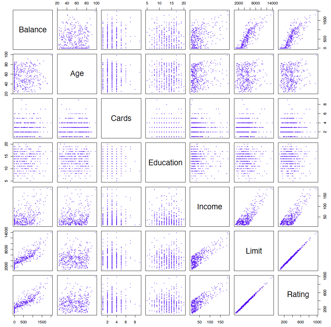
See for example the scatterplot matrix of the credit card data in the following figure.
例如，请参见下图中信用卡数据的散点图矩阵。

In addition to the 7 quantitative variables shown, there are four qualitative variables: gender, student (student status), status (marital status), and ethnicity (Caucasian, African American (AA) or Asian).
除了所示的 7 个定量变量外，还有四个定性变量：性别、学生（学生身份）、状态（婚姻状况）和种族（高加索人、非裔美国人（AA）或亚裔）。

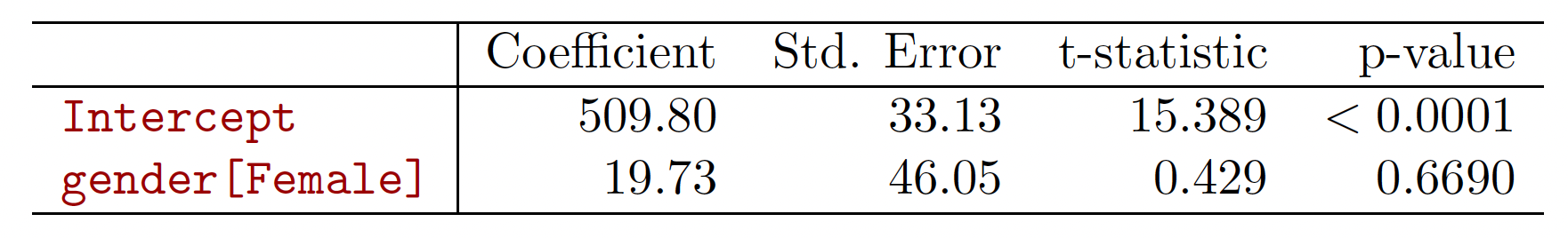
Example: investigate differences in credit card balance between males and females, ignoring the other variables. We create a new dummy variable
示例：调查男女之间信用卡余额的差异，忽略其他变量。我们创建一个新的伪变量

x_i = \begin{cases} 1 \mbox{, if $i$th person is female} \\ 0\mbox{, if $i$th person is not female} \end{cases}

Resulting model:
结果模型：

y_i=\beta_0+\beta_1x_i +\epsilon = \begin{cases} \beta_0+\beta_1+\epsilon_i \mbox{, if $i$th person is female} \\ \beta_0+\epsilon_i \mbox{, if $i$th person is not female} \end{cases}

Interpretation?
解释如下

$\beta_0$ = average $Y$ among non-females
$\beta_0+\beta_1$ = average $Y$ among females
$\beta_1$ average difference in $Y$ between the two groups.

Results for gender model:

With more than two levels, we create additional dummy variables.
对于两个以上的级别，我们创建额外的虚拟变量。

For example, for the ethnicity variable we create two dummy variables.
例如，对于种族变量，我们创建了两个虚拟变量。

The first could be
第一个可能是

x_{i1} = \begin{cases} 1 \mbox{, if $i$th person is Asian} \\ 0\mbox{, if $i$th person is not Asian} \end{cases}

and the second could be
第二种可能是

x_{i2} = \begin{cases} 1 \mbox{, if $i$th person is Caucasian} \\ 0\mbox{, if $i$th person is not Caucasian} \end{cases}

Then both of these variables can be used in the regression equation, in order to obtain the model
然后这两个变量都可以用于回归方程中，以获得模型

$y_{i}=\beta_{0}+\beta_{1} x_{i 1}+\beta_{2} x_{i 2}+\epsilon_{i}=\left\{\begin{array}{ll} \beta_{0}+\beta_{1}+\epsilon_{i} & \text { if } i \text { th person is Asian } \\ \beta_{0}+\beta_{2}+\epsilon_{i} & \text { if } i \text { th person is Caucasian } \\ \beta_{0}+\epsilon_{i} & \text { if } i \text { th person is AA } \end{array}\right.$

There will always be one fewer dummy variable than the number of levels.
虚拟变量总是比级别数少一个。

The level with no dummy variable
没有虚拟变量的级别

African American in this example --- is known as the baseline.
在这个例子中，非洲裔美国人被称为基线。

# Qualitative predictors in R R 中的定性预测变量

How to create dummy variable in R ?
如何在 R 中创建虚拟变量？

We use a date set Salaries from package carData
我们使用 carData 包中的日期集 Salaries

	# Load the data
	data("Salaries", package = "carData")
	summary(Salaries)

        rank     discipline yrs.since.phd    yrs.service        sex     
 AsstProf : 67   A:181      Min.   : 1.00   Min.   : 0.00   Female: 39  
 AssocProf: 64   B:216      1st Qu.:12.00   1st Qu.: 7.00   Male  :358  
 Prof     :266              Median :21.00   Median :16.00               
                            Mean   :22.31   Mean   :17.61               
                            3rd Qu.:32.00   3rd Qu.:27.00               
                            Max.   :56.00   Max.   :60.00               
     salary      
 Min.   : 57800  
 1st Qu.: 91000  
 Median :107300  
 Mean   :113706  
 3rd Qu.:134185  
 Max.   :231545

# Qualitative predictors with two levels 两级定性预测变量

If we use sex as an argument in lm , R will correctly treat sex as single dummy variable with two categories.
如果我们在 lm 中使用 sex 作为参数，R 将正确地将 sex 视为具有两个类别的单个伪变量。

	md1<-lm(salary~sex,data = Salaries)
	summary(md1)

Call:
lm(formula = salary ~ sex, data = Salaries)

Residuals:
   Min     1Q Median     3Q    Max 
-57290 -23502  -6828  19710 116455 

Coefficients:
            Estimate Std. Error t value Pr(>|t|)    
(Intercept)   101002       4809  21.001  < 2e-16 ***
sexMale        14088       5065   2.782  0.00567 ** 
---
Signif. codes:  0 '***' 0.001 '**' 0.01 '*' 0.05 '.' 0.1 ' ' 1

Residual standard error: 30030 on 395 degrees of freedom
Multiple R-squared:  0.01921,   Adjusted R-squared:  0.01673 
F-statistic: 7.738 on 1 and 395 DF,  p-value: 0.005667

# Qualitative predictors with more than two levels 两级以上的定性预测变量

What about the categorical data with more than two levels?

As rank is a factor with three levels, R automatically create two dummy variables.
由于 rank 是一个具有三个级别的 factor ， R 会自动创建两个虚拟变量。

	md2<-lm(salary~rank,data = Salaries)
	summary(md2)

Call:
lm(formula = salary ~ rank, data = Salaries)

Residuals:
   Min     1Q Median     3Q    Max 
-68972 -16376  -1580  11755 104773 

Coefficients:
              Estimate Std. Error t value Pr(>|t|)    
(Intercept)      80776       2887  27.976  < 2e-16 ***
rankAssocProf    13100       4131   3.171  0.00164 ** 
rankProf         45996       3230  14.238  < 2e-16 ***
---
Signif. codes:  0 '***' 0.001 '**' 0.01 '*' 0.05 '.' 0.1 ' ' 1

Residual standard error: 23630 on 394 degrees of freedom
Multiple R-squared:  0.3943,    Adjusted R-squared:  0.3912 
F-statistic: 128.2 on 2 and 394 DF,  p-value: < 2.2e-16

Question: What is the baseline here?

# In-Calss Exercise

Please construct a simple linear regression model to predict salary by discipline .
请构造一个简单的线性回归模型，根据 discipline 预测 salary 。

	# Load the data
	data("Salaries", package = "carData")
	slm <-lm(salary~discipline, data= Salaries)
	summary(slm)

## 
## Call:
## lm(formula = salary ~ discipline, data = Salaries)
## 
## Residuals:
##    Min     1Q Median     3Q    Max 
## -50748 -24611  -4429  19138 113516 
## 
## Coefficients:
##             Estimate Std. Error t value Pr(>|t|)    
## (Intercept)   108548       2227  48.751  < 2e-16 ***
## disciplineB     9480       3019   3.141  0.00181 ** 
## ---
## Signif. codes:  0 '***' 0.001 '**' 0.01 '*' 0.05 '.' 0.1 ' ' 1
## 
## Residual standard error: 29960 on 395 degrees of freedom
## Multiple R-squared:  0.02436,    Adjusted R-squared:  0.02189 
## F-statistic: 9.863 on 1 and 395 DF,  p-value: 0.001813

Please construct a multiple linear regression model to predict salary with yrs.sevice , rank , and sex .
请构建一个多元线性回归模型，用 yrs.sevice 、 rank 和 sex 预测 salary
Hint You can use + to connect the attributes/features.
提示可以使用 + 连接属性 / 功能

	mlm <- lm(salary~yrs.service + rank + sex, data= Salaries)
	summary(mlm)

## 
## Call:
## lm(formula = salary ~ yrs.service + rank + sex, data = Salaries)
## 
## Residuals:
##    Min     1Q Median     3Q    Max 
## -64500 -15111  -1459  11966 107011 
## 
## Coefficients:
##               Estimate Std. Error t value Pr(>|t|)    
## (Intercept)    76612.8     4426.0  17.310  < 2e-16 ***
## yrs.service     -171.8      115.3  -1.490  0.13694    
## rankAssocProf  14702.9     4266.6   3.446  0.00063 ***
## rankProf       48980.2     3991.8  12.270  < 2e-16 ***
## sexMale         5468.7     4035.3   1.355  0.17613    
## ---
## Signif. codes:  0 '***' 0.001 '**' 0.01 '*' 0.05 '.' 0.1 ' ' 1
## 
## Residual standard error: 23580 on 392 degrees of freedom
## Multiple R-squared:    0.4,  Adjusted R-squared:  0.3938 
## F-statistic: 65.32 on 4 and 392 DF,  p-value: < 2.2e-16

# Extensions of the linear model 线性模型的扩展

What is wrong with the linear model? It works quite well!

Yes -- but sometimes the (restrictive) assumptions are violated in practice.
但在实践中，有时会违背 (限制性的) 假设。

Assumption 1: additivity 假设 1：可加性: The relationship between the predictors and response is additive.
预测变量和响应变量之间的关系是相加的。
effect of changes in a predictor $X_j$ on the response $Y$ is independent of the values of the other predictors.
预测变量 $X_j$ 的变化，对响应变量 $Y$ 的影响，与其他预测的值无关。
Assumption 2: linearity 假设 2: 线性: The relationship between the predictors and response is linear.
预测变量和响应变量之间的关系线性的。
the change in the response $Y$ due to a one-unit change in $X_j$ is constant, regardless of the value of $X_j$ .
无论 $X_j$ 的值是多少，由于 $X_j$ 的一个单位变化而导致的响应变量 $Y$ 的变化是恒定的。

# Removing the additive assumption 去掉加性假设

Previous analysis of Advertising data: both TV and radio seem associated with sales.
之前对 Advertising 数据的分析： TV 和 radio 似乎都与销售额有关。

The linear models that formed the basis for this conclusion:
构成这一结论基础的线性模型：

$sales=\beta_0+ \beta_1 TV + \beta_2 radio + \beta_3 newspaper +\epsilon$

The above model states that the average effect on sales of a one-unit increase in TV is always $\beta_1,$ regardless of the amount spent on radio.
上面的模型表明，tv 每增加一个单位对销售额的平均影响总是 $\beta_1$ ，无论花在 radio 上的金额是多少。

But suppose that spending money on radio advertising actually increases the effectiveness of TV advertising, so that the slope term for TV should increase as radio increases.
但假设把钱花在广播广告上实际上提高了电视广告的效果，那么电视的斜率应该随着广播的增加而增加。

In this situation, given a fixed budget of $100,000, spending half on radio and half on TV may increase sales more than allocating the entire amount to either TV or to radio.
在这种情况下，考虑到 10 万美元的固定预算，一半用于广播，一半用于电视，可能会增加销售额，而不是将全部资金分配给电视或广播。

In marketing, this is known as a synergy effect, and in statistics it is referred to as an interaction effect.
在市场营销中，这被称为协同效应，在统计学中，这被称为互动效应。

We will now explain how to augment this model by allowing interaction between radio and TV in predicting sales :
现在，我们将解释如何通过允许 radio 和 TV 在预测 “销售额” sales 时进行交互来扩展此模型：

$sales =\beta_0+\beta_1\times TV+\beta_2\times radio +\beta_3 \times (radio\times TV)+\epsilon\\ = \beta_0+ \textcolor{blue}{(\beta_1+\beta_3\times radio)\times TV} + \beta_2\times radio + \epsilon.$

# Interpretation

$\beta_3$ = increase in the effectiveness of TV advertising for a one unit increase in radio advertising (or vice-versa).
电视广告的有效性增加一个单位，广播广告增加一个单位（反之亦然）。

Interpretation

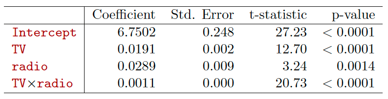
The results in this table suggests that interactions are
important.
此表中的结果表明相互作用很重要。
The p-value for the interaction term TV $\times$ radio is extremely low, indicating that there is strong evidence for $H_A : \beta_3\ne 0.$
交互术语 TV $\times$ radio 的 p 值极低，表明有充分证据表明 $H_A : \beta_3\ne 0.$
The R2 for the interaction model is 96.8%, compared to only 89.7% for the model that predicts sales using TV and radio without an interaction term.
互动模型的 R2 为 96.8%，相比之下，不使用互动术语预测电视和广播销售的模型仅为 89.7%。

# Hierarchy Principle 等级原则

Sometimes it is the case that an interaction term has a very small p-value, but the associated main effects (in this case, TV and radio) do not.
有时交互项的 p 值很小，但相关的主要效果 (在本例中是电视和收音机) 却没有。

If we include an interaction in a model, we should also include the main effects, even if the p-values associated with their coefficients are not significant.
如果我们在模型中包括交互作用，我们也应该包括主要影响，即使与其系数相关的 p 值并不显著。

The rationale for this principle is that interactions are hard to interpret in a model without main effects --- their meaning is changed.
这个原则的基本原理是，在没有主要影响的模型中，交互很难被解释 —— 它们的意义被改变了。

Specifically, the interaction terms also contain main effects, if the model has no main effect terms.
具体来说，如果模型没有主效应项，交互项也包含主效应。

We can also have the interactions between qualitative and quantitative variables.
我们也可以有定性和定量变量之间的相互作用。

Consider the Credit data set, and suppose that we wish to predict balance using income (quantitative) and student (qualitative).
考虑一下 Credit 数据集，假设我们希望用 income (定量) 和 student (定性) 来预测平衡。

Without an interaction term, the model takes the form
如果没有交互项，模型就会采用

$\begin{aligned} \text { balance }_{i} & \approx \beta_{0}+\beta_{1} \times \text { income }_{i}+\left\{\begin{array}{ll} \beta_{2} & \text { if } i \text { th person is a student } \\ 0 & \text { if } i \text { th person is not a student } \end{array}\right.\\ &=\beta_{1} \times \text { income }_{i}+\left\{\begin{array}{ll} \beta_{0}+\beta_{2} & \text { if } i \text { th person is a student } \\ \beta_{0} & \text { if } i \text { th person is not a student. } \end{array}\right. \end{aligned}$

With interactions, it takes the form
有交互项，则

$\begin{aligned} \text { balance }_{i} & \approx \beta_{0}+\beta_{1} \times \text { income }_{i}+\left\{\begin{array}{ll} \beta_{2}+\beta_{3} \times \text { income }_{i} & \text { if student } \\ 0 & \text { if not student } \end{array}\right.\\ &=\left\{\begin{array}{ll} \left(\beta_{0}+\beta_{2}\right)+\left(\beta_{1}+\beta_{3}\right) \times \text { income }_{i} & \text { if student } \\ \beta_{0}+\beta_{1} \times \text { income }_{i} & \text { if not student } \end{array}\right. \end{aligned}$

For the Credit data, the least squares lines are shown for prediction of balance from income for students and non-students.
对于信用数据，显示了最小二乘线，用于预测学生和非学生的收入平衡。

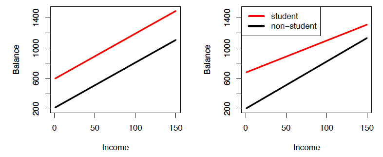
Left: The model was fit. There is no interaction between income and student.
这个模型很合适。收入和学生之间没有交互作用。

Right: The model was fit. There is an interaction term between income and student.
右图：模型很合适。收入和学生之间有一个互动术语。

# Interaction in R R 中的相互作用

Let's revisit the auto data set. Here we want to build a model as follows.
在这里，我们要建立一个模型，如下。

$mpg = \beta_0 + \beta_1 \times horsepower + \beta_2 \times horsepower^2 + \epsilon$

How to do it in R?

	horsepowerSquare <- Auto$horsepower * Auto$horsepower
	interModel1 <- lm(mpg~ horsepower + horsepowerSquare, Auto)
	summary(interModel1)

Call:
lm(formula = mpg ~ horsepower + horsepowerSquare, data = Auto)

Residuals:
     Min       1Q   Median       3Q      Max 
-14.7135  -2.5943  -0.0859   2.2868  15.8961 

Coefficients:
                   Estimate Std. Error t value Pr(>|t|)    
(Intercept)      56.9000997  1.8004268   31.60   <2e-16 ***
horsepower       -0.4661896  0.0311246  -14.98   <2e-16 ***
horsepowerSquare  0.0012305  0.0001221   10.08   <2e-16 ***
---
Signif. codes:  0 '***' 0.001 '**' 0.01 '*' 0.05 '.' 0.1 ' ' 1

Residual standard error: 4.374 on 389 degrees of freedom
Multiple R-squared:  0.6876,    Adjusted R-squared:  0.686 
F-statistic:   428 on 2 and 389 DF,  p-value: < 2.2e-16

Actaully, if it is the interaction with two different features, we just need to use * .
事实上，如果是两个不同特征的交互，我们只需要使用 * 。

For example, we want to check the interactions between horsepower and weight .
例如，我们要检查 horsepower 和 weight 之间的相互作用。

	interModel2 <- lm(mpg~ horsepower * weight, Auto)
	summary(interModel2)

Call:
lm(formula = mpg ~ horsepower * weight, data = Auto)

Residuals:
     Min       1Q   Median       3Q      Max 
-10.7725  -2.2074  -0.2708   1.9973  14.7314 

Coefficients:
                    Estimate Std. Error t value Pr(>|t|)    
(Intercept)        6.356e+01  2.343e+00  27.127  < 2e-16 ***
horsepower        -2.508e-01  2.728e-02  -9.195  < 2e-16 ***
weight            -1.077e-02  7.738e-04 -13.921  < 2e-16 ***
horsepower:weight  5.355e-05  6.649e-06   8.054 9.93e-15 ***
---
Signif. codes:  0 '***' 0.001 '**' 0.01 '*' 0.05 '.' 0.1 ' ' 1

Residual standard error: 3.93 on 388 degrees of freedom
Multiple R-squared:  0.7484,    Adjusted R-squared:  0.7465 
F-statistic: 384.8 on 3 and 388 DF,  p-value: < 2.2e-16

Question: Why I don't need to + horsepower + weight ?
为什么不需要 + horsepower + weight ?

We can use the same way to construct interaction regression model with one numeric attribute and one categorical attribute.
我们可以用同样的方法构造一个数值属性和一个范畴属性的交互式回归模型。

Note: Only when these two features have interactions, our interactions model can lead to a better performance.
注意：只有当这两个特性有交互时，我们的交互模型才能导致更好的性能。

# In-Calss Exercise:

Please construct an interaction regression model to predict salary with yrs.service and yrs.since.phd for the Salaries data set.
请建立一个交互式回归模型，通过 yrs.service 和 yrs.since.phd ，为 Salaries 数据集预测 salary 。

	interlm <-lm(salary~ yrs.service* yrs.since.phd, data= Salaries)
	summary(interlm)

## 
## Call:
## lm(formula = salary ~ yrs.service * yrs.since.phd, data = Salaries)
## 
## Residuals:
##    Min     1Q Median     3Q    Max 
## -63823 -17292  -2538  13158 107001 
## 
## Coefficients:
##                            Estimate Std. Error t value Pr(>|t|)    
## (Intercept)               70155.263   3472.077  20.206  < 2e-16 ***
## yrs.service                1692.446    356.279   4.750 2.85e-06 ***
## yrs.since.phd              2194.289    246.862   8.889  < 2e-16 ***
## yrs.service:yrs.since.phd   -64.617      7.487  -8.630  < 2e-16 ***
## ---
## Signif. codes:  0 '***' 0.001 '**' 0.01 '*' 0.05 '.' 0.1 ' ' 1
## 
## Residual standard error: 25120 on 393 degrees of freedom
## Multiple R-squared:  0.3177, Adjusted R-squared:  0.3125 
## F-statistic: 60.99 on 3 and 393 DF,  p-value: < 2.2e-16

Please construct an interaction regression model to predict salary with yrs.service and rank for the Salaries data set.
Note rank is a categorical feature.
请建立一个交互式回归模型，用 yrs.service 和 rank 来为 Salaries 数据集预测 salary 。

	interlm2 <- lm(salary~ yrs.service*rank, data= Salaries)
	summary(interlm2)

## 
## Call:
## lm(formula = salary ~ yrs.service * rank, data = Salaries)
## 
## Residuals:
##    Min     1Q Median     3Q    Max 
## -65609 -15841  -1047  11177 106585 
## 
## Coefficients:
##                           Estimate Std. Error t value Pr(>|t|)    
## (Intercept)                78926.6     5445.1  14.495  < 2e-16 ***
## yrs.service                  779.3     1945.2   0.401  0.68891    
## rankAssocProf              19667.6     7127.5   2.759  0.00606 ** 
## rankProf                   50567.8     6318.2   8.004 1.39e-14 ***
## yrs.service:rankAssocProf  -1174.0     1967.4  -0.597  0.55104    
## yrs.service:rankProf        -898.6     1949.2  -0.461  0.64505    
## ---
## Signif. codes:  0 '***' 0.001 '**' 0.01 '*' 0.05 '.' 0.1 ' ' 1
## 
## Residual standard error: 23640 on 391 degrees of freedom
## Multiple R-squared:  0.3986, Adjusted R-squared:  0.391 
## F-statistic: 51.84 on 5 and 391 DF,  p-value: < 2.2e-16

	interlm2 <-lm(salary~ yrs.service* yrs.since.phd + rank, data= Salaries)
	summary(interlm2)

## 
## Call:
## lm(formula = salary ~ yrs.service * yrs.since.phd + rank, data = Salaries)
## 
## Residuals:
##    Min     1Q Median     3Q    Max 
## -53996 -16032  -2237  12039 107358 
## 
## Coefficients:
##                            Estimate Std. Error t value Pr(>|t|)    
## (Intercept)               76090.368   3408.690  22.322  < 2e-16 ***
## yrs.service                 479.244    394.043   1.216   0.2246    
## yrs.since.phd               761.967    314.188   2.425   0.0158 *  
## rankAssocProf              7031.646   5056.227   1.391   0.1651    
## rankProf                  36534.191   6057.562   6.031 3.77e-09 ***
## yrs.service:yrs.since.phd   -24.656      9.639  -2.558   0.0109 *  
## ---
## Signif. codes:  0 '***' 0.001 '**' 0.01 '*' 0.05 '.' 0.1 ' ' 1
## 
## Residual standard error: 23440 on 391 degrees of freedom
## Multiple R-squared:  0.4088, Adjusted R-squared:  0.4012 
## F-statistic: 54.07 on 5 and 391 DF,  p-value: < 2.2e-16

# Potential problems 潜在的问题

# Common issues and problems 共同的问题和困难

Non-linearity of the response-predictor relationships.
响应 - 预测关系的非线性。
Correlation of error terms.
误差项的相关性。
Non-constant variance of error terms.
误差项的非常数方差。
Outliers. 异常值
High-leverage points. 高杠杆点。
Collinearity 共线性

# Reference

Probability & Statistics for Engineers & Scientist, 9th Edition, Ronald E. Walpole, Raymond H. Myers, Sharon L. Myers, Keying Ye, Prentice Hall
Chapter 3 of the textbook Gareth James, Daniela Witten, Trevor Hastie and Robert Tibshirani, An Introduction to Statistical Learning: with Applications in R.
Part of this lecture notes are extracted from Prof. Sonja Petrovic ITMD/ITMS 514 lecture notes.

Python R