# Objective

• What is a 'regression' function
  什么是 “回归” 函数
• Simple linear regression
  简单线性回归
• Best approximation, least squares, residual sum of squares (RSS), RSE, $R^2$
  最佳近似、最小二乘法、残差平方和 (RSS)、RSE、$R^2$
• Understand the output of a simple linear regression
  理解简单线性回归的输出
• Basic R and Python command to run a simple linear regression model
  用基本的 R 和 Python 命令运行简单线性回归模型

# Advertising Example

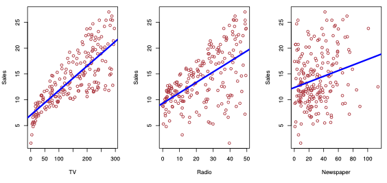
Figure 2.1. from ISLR: Y = Sales plottedagainst TV , Radio and Newspaper advertising budgets.
来自 ISLR：Y = Sales ，根据 TV 、 Radio 和 Newspper 三种途径的广告预算绘制。

Our goal is to develop an accurate model ($f$) that can be used to predict sales on the basis of the three media budgets:
我们的目标是开发一个准确的模型 ($f$)，可以用来根据三种媒体预算预测 sales 销售额：

$$Sales \approx f(TV, Radio, Newspaper).$$

• Sales = a reponse, target, or outcome.
  Sales 是响应、目标、或结果。

  • The variable we want to predicit.
    是我们想要预测的变量。
  • Denoted by $Y$.
    用$Y$ 表示。

• TV is one of the features, or inputs.
  TV 是特征之一，或输入。

  • Denoted by $X_1$.
    用$X_1$ 表示。

• Similarly for Radio and Newspaper .
  另外两者也类似

• We can put all the predictors into a single input vector
  我们可以将所有的预测变量放入一个输入向量中

  $$X = (X_1,X_2,X_3)$$

• Now we can write our model as
  现在我们可以将我们的模型写成

  $$Y=f(X) +\epsilon$$

  , where $\epsilon$ captures measurement errors and other discrepancies between the response $Y$ and the model $f$.
  其中 $\epsilon$ 捕获测量误差，以及响应变量$Y$ 和模型$f$ 之间的其他差异。

# Regression function 回归函数

Formally, the regression function is given by $E(Y | X = x)$. This is the expected value of $Y$ at $X = x$.
形式上，回归函数由 $E(Y | X = x)$ 给出。这是$Y$ 在 $X = X$ 时的期望值。
The ideal or optimal predictor of $Y$ based on $X$ is thus
基于$X$，$Y$ 的理想或最佳预测变量是这样的

$$f(x) = E(Y | X = x)$$

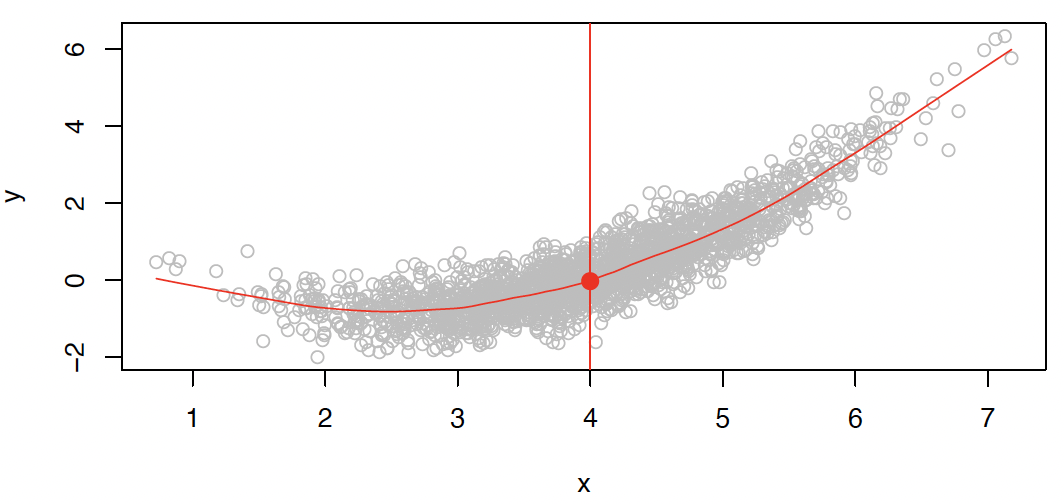
A good value is $$ f(4) = E(Y | X = 4) $$

# Simple linear regression using a single predictor $X$ 使用单一预测值的简单线性回归 $X$

• Predict a quantitative $Y$ by single predictor variable $X$
  通过单个预测变量$X$ 预测一个定量的$Y$

$$Y \approx \beta_0+\beta_1 X$$

• Example: $sales \approx \beta_0+\beta_1\times TV$.

• $\beta_0$, $\beta_1$ are two unknown constants that represent the intercept and slope. [parameters, or coefficients.]
  $\beta_0$ 和 $\beta_1$ 是两个未知常数，分别表示截距和斜率。(参数或系数。)

Prediction

$$\hat y = \hat\beta_0+\hat\beta_1x.$$

# How to estimate the coefficients 如何估计系数

Let $\hat{y}_i = \hat\beta_0+\hat\beta_1x_i$ be the prediction for $Y$ based on the $i$th value of $X$.
基于$X$ 的第$i$ 个值，对$Y$ 的预测。

$e_i = y_i-\hat{y}_i$ represents the $i$th residual.
代表了第$i$ 个剩余。

Residual Sum of Squares RSS 剩余平方和

$$\text{RSS} = \sum_{i=1}^n e_i^2 = \sum_{i=1}^n(y_i-\hat{y}_i)^2.$$

The least squares approach chooses $\beta_0$ and $\beta_1$ to minimize RSS.
最小二乘法选择 $\beta_0$ 和 $\beta_1$ 来最小化 RSS。

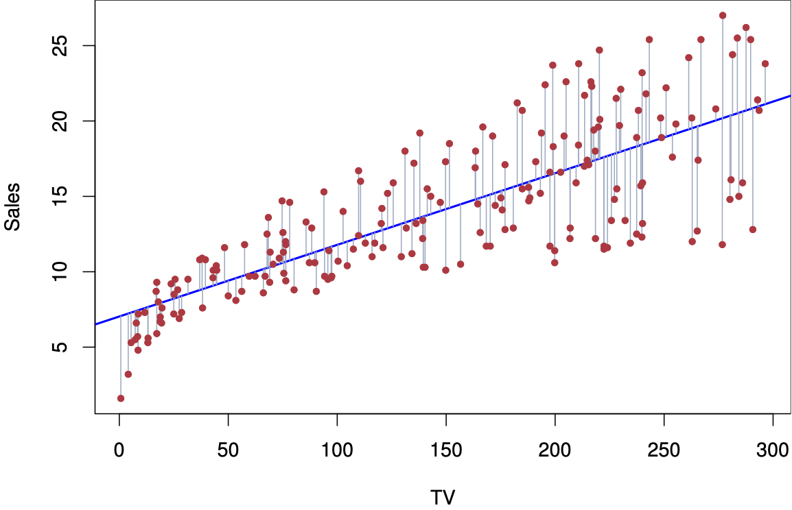
Fig 3.1. ISLR: For the Advertising data, the least squares fit for the regression of sales onto TV is shown.
对于 Advertising 数据，显示了 sales 与 TV 回归的最小二乘法。

The fit is found by minimizing the sum of squared errors.
拟合是通过最小化误差平方和来找到的。

Each grey line segment represents an error, and the fit makes a compro- mise by averaging their squares.
每个灰色线段代表一个误差，拟合通过平均它们的平方来做出妥协。

In this case a linear fit captures the essence of the relationship, although it is somewhat deficient in the left of the plot.
在这种情况下，线性拟合抓住了关系的本质，尽管它在图的左侧有些不足。

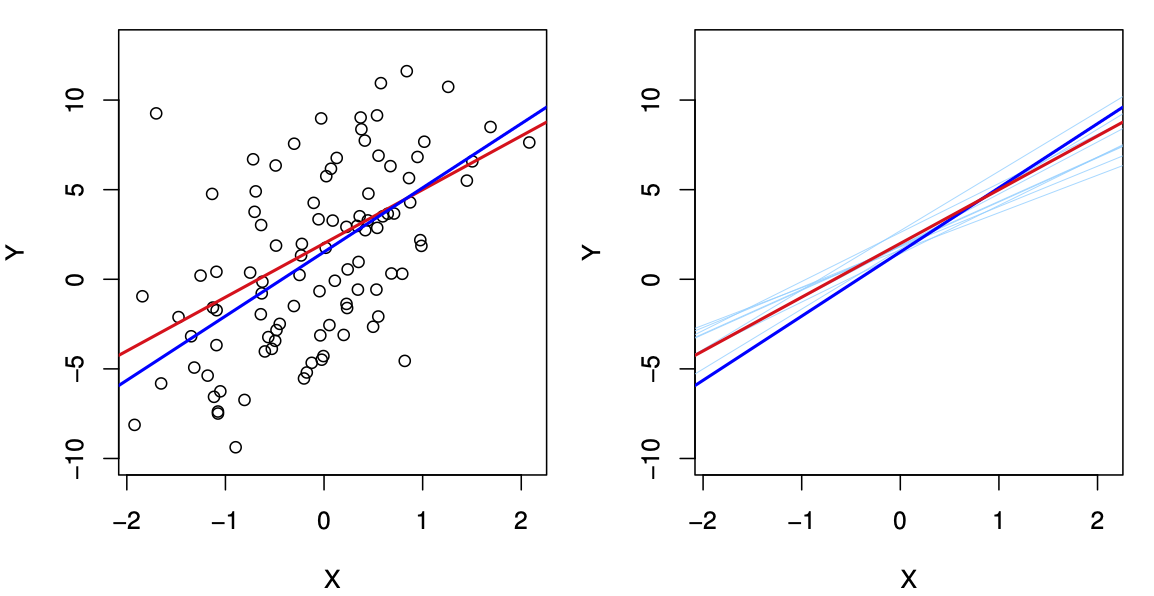
Fig. 3.2. ISLR: A simulated data set.
一个模拟数据集。

Left: The red line represents the true relationship, $f(X) = 2 + 3X$, which is known as the population regression line.
红线表示真实的关系，也就是总体回归线。

The blue line is the least squares line; it is the least squares estimate for $f(X)$ based on the observed data, shown in black.
蓝线是最小二乘线；它是基于观测数据的 $f(X)$ 的最小二乘估计，用黑色显示。

Right: The population regression line is again shown in red, and the least squares line in dark blue.
右图：总体回归线再次显示为红色，最小二乘线显示为深蓝色。

In light blue, ten least squares lines are shown, each computed on the basis of a separate random set of observations.
用浅蓝色表示十条最小平方线，每条线都是根据一组随机的观测数据计算出来的。

Each least squares line is different, but on average, the least squares lines are quite close to the population regression line.
每条最小二乘线不同，但平均而言，最小二乘线与总体回归线非常接近。

# Understand the output 了解输出

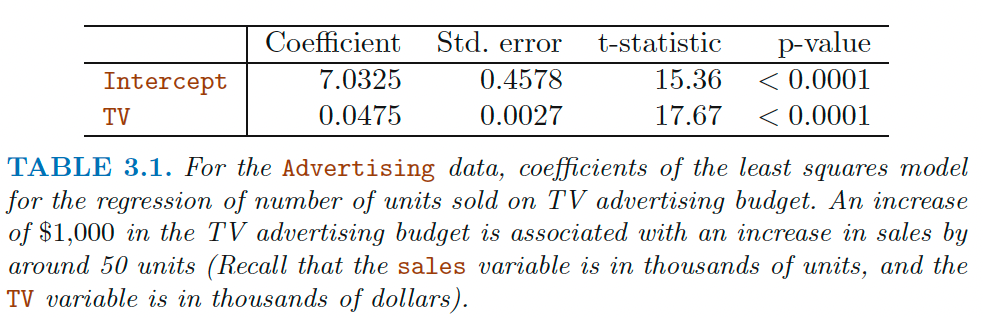
For the Advertising data, coefficients of the least squares modei for the regression of number of units sold on TV advertising budget.
对于广告数据，回归电视广告预算中销售单位数量的最小二乘模型系数。

An increase of $1,000 in the TV advertising budget is associated with an increase in sales by around 50 units (Recall that the sales variable is in thousands of units, and the TV variable is in thousands of dollars).
电视广告预算增加 1000 美元与销售增加约 50 个单位有关（回想一下，销售变量以千单位为单位，电视变量以千美元为单位）。

Here $t= \frac{\hat \beta_i-0}{SE(\hat\beta_i)}$ is a t statistic. 是一个 t 统计

Question: Is there a relationship between the response $Y$ and predictor $X$?
响应变量$Y$ 和预测变量$X$ 之间有关系吗？

We can do a hypothesis testing.
我们可以做一个假设检验。

• check whether $\beta_1=0$

  • Hypothesis test: $H_0:\beta_1=0$ vs. $H_1: \beta_1\neq 0$.
  • a $t$-statistic measures the number of standard deviations that $\beta_1$ is away from 0 (specifically, $t= \frac{\hat \beta_1-0}{SE(\hat\beta_1)}$ with $n-2$ degrees of freedom)
    $t$ - 统计测量 \BETA_1 远离 0 的标准偏差数（具体地说，$t= \frac{\hat \beta_1-0}{SE(\hat\beta_1)}$，自由度为 $n-2$）

• $p$-value

  • the probability of observing any value equal to t or larger; as usual! - the probability of seeing the data we saw under the $H_0$
    观察到等于或大于 t 的任何值的概率；像往常一样！- 看到我们在$H_0$ 下看到的数据的概率

  • in practice, we just read off the $t$-test. or read off the output of linear models.
    实际上，我们只是读出了$t$-test。或读出线性模型的输出。

# Assessing model fit 评定模型拟合

Question: Suppose we have rejected the null hypothesis in favor of the alternative. Now what??
问题：假设我们拒绝了无效假设，支持另一种假设，现在怎么办？

• Natural: quantify the extent to which the model fits the data.
  自然的：量化模型适合数据的程度。
• The quality of a linear regression fit is typically assessed using two related quantities:
  线性回归拟合的质量通常使用两个相关量进行评估：
  • the residual standard error RSE and
    残差标准误差 RSE
  • the $R^2$ statistic.
    $R^2$ 统计

Advertising Data Results

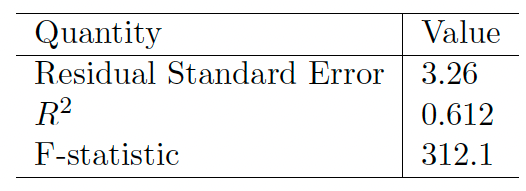
# RSE

A measure of the lack of fit of the model simple linear regression model to the data:
一种衡量模型拟合不足的方法简单线性回归模型对数据的拟合:

$$RSE = \sqrt{\frac{1}{n-2}RSS} = \sqrt{\frac{1}{n-2}\sum_{i=1}^n (y_i-\hat y_i)^2}$$

• If the predictions obtained using the model are very close to the true outcome values ($\hat y_i\approx y_i$ for i = 1, ..., n), then RSE will be small
  如果使用模型得到的预测非常接近真实的结果值 ($\hat y_i\approx y_i$ for i = 1, ..., n)，则 RSE 将很小

  • we can conclude that the model fits the data very well.
    我们可以得出结论，这个模型与数据吻合得很好。

• If $\hat y_i$ is very far from $y_i$ for one or more observations, then the RSE may be quite large
  如果 $\hat y_i$ 与 $y_i$ 之间有很大的距离，那么 RSE 可能相当大

  • indicating that the model doesn’t fit the data well.
    这表明模型与数据的拟合并不好。

Interpretation 解释
The RSE provides an absolute measure of lack of fit.
RSE 提供了一种绝对的缺乏契合度的测量方法。

But since it is measured in the units of $Y$ , it is not always clear what constitutes a good RSE...
但由于它是以$Y$ 为单位来衡量的，所以并不总是清楚什么构成了一个好的 RSE……

# $R^2$

The $R^2$ statistic provides an alternative measure of fit (proportion):
$R^2$ 统计提供了另一种拟合方法 (比例):

$$R^2 = \frac{TSS-RSS}{TSS}=1 - \frac{RSS}{TSS}$$

• TSS = total sum of squares $\sum_{i=1}^n(y_i-\bar y)^2$
  where $\bar y = \frac{1}{n}\sum_{i=1}^ny_i$
  总平方和
• RSS = residual sum of squares $\sum_{i=1}^n(y_i-\hat y_i)^2$
  残差平方和

$R^2$ measures the proportion of variability in $Y$ that can be explained using $X$
$R^2$ 衡量的是可以用$X$ 解释的$Y$ 的可变性比例

Interpretation 解释
Always between 0 and 1 (independent of scale of $Y$).
总是在 0 和 1 之间 (与$Y$ 的比例无关)。

Question What's a good value?
问题是什么样的才算是良好的值
Can be challenging to determine ... in general, depends on the application.
很难确定… 一般来说，取决于应用程序。

# How to construct linear regression in R

Use simple linear regression on the Auto data set.
对 Auto 数据集使用简单的线性回归。

• Use the lm() function to perform a simple linear regression with mpg as the response and horsepower as the predictor.
  使用 lm() 函数执行一个简单的线性回归，以 mpg 作为响应变量， horsepower 作为预测变量。

  require(ISLR)

  Loading required package: ISLR
  

  	data(Auto)
  	fitlm <- lm(mpg ~ horsepower, data=Auto)

Where is the output??

• Let's take a look at the fitlm object.
  Use the summary() function to print the results.

  summary(fitlm)

  Call:
  lm(formula = mpg ~ horsepower, data = Auto)
  
  Residuals:
      Min       1Q   Median       3Q      Max 
  -13.5710  -3.2592  -0.3435   2.7630  16.9240 
  
  Coefficients:
              Estimate Std. Error t value Pr(>|t|)    
  (Intercept) 39.935861   0.717499   55.66   <2e-16 ***
  horsepower  -0.157845   0.006446  -24.49   <2e-16 ***
  ---
  Signif. codes:  0 '***' 0.001 '**' 0.01 '*' 0.05 '.' 0.1 ' ' 1
  
  Residual standard error: 4.906 on 390 degrees of freedom
  Multiple R-squared:  0.6059,    Adjusted R-squared:  0.6049 
  F-statistic: 599.7 on 1 and 390 DF,  p-value: < 2.2e-16
  

• Is there a relationship between the predictor and the response?
  预测变量和响应变量之间有关系吗？

  • Yes

• How strong is the relationship between the predictor and the response?
  预测变量和响应变量之间的关系有多强？

  • $p$-value is close to 0: relationship is strong
    $p$-value 接近 0：关系强

• Is the relationship between the predictor and the response positive or negative?
  预测变量和响应变量之间的关系是积极的还是消极的？

  • Coefficient is negative: relationship is negative
    系数为负：关系为负

• What is the predicted mpg associated with a horsepower of $98$? What are the associated 95% confidence and prediction intervals?
  $98$ 的被预测的 mpg 对应的 horsepower 是多少？相关的 95% 置信和预测区间是什么？

First you have to make a new data frame object which will contain the new point:
首先，你必须创建一个新的数据帧对象，它将包含新的点:

new <- data.frame(horsepower = 98)

predict(fitlm, new) # predicted mpg

       1 
24.46708 

predict(fitlm, new, interval="confidence") # conf interval

       fit      lwr      upr
1 24.46708 23.97308 24.96108

predict(fitlm, new, interval="prediction") # pred interval

       fit     lwr      upr
1 24.46708 14.8094 34.12476

What is the difference between confidence and prediction intervals!? $\rightarrow$ we will learn in the next lecture!!
置信区间和预测区间有什么区别？

# How to construct linear regression in Python

library(reticulate)

# import the necessary packages

import pandas as pd

import numpy as np

import statsmodels.api as sm #py_install("statsmodels")

We still want to find the relationship between mpg and horsepower . Let's read the dataset first.
我们仍然想要找到 mpg 和 horsepower 之间的关系。
让我们先阅读数据集。

# Read the data set from the website of our textbook

auto = pd.read_csv('https://www.statlearning.com/s/Auto.csv')

# Here I dropped the records with horsepower = ?

auto = auto.drop(labels=[32,126,330,336,354], axis=0)

# choose the predictor

# 选择预测变量

X = auto[['horsepower']]

# choose the response

# 选择响应变量

y = auto[['mpg']]

# add a constant to the predictor

# 向预测变量添加一个常数

X = sm.add_constant(X)

# OLS stands for “Ordinary Least Squares”

# OLS 代表普通最小二乘

# `horsepower` consider as a object, so I use astype to convert it to numeric

# `horsepower` 考虑作为一个对象，所以使用 astype 将它转换为数字

model01 = sm.OLS(y, X.astype(float)).fit()

# To obtain the results of the regression model, run the `summary()` command on the model

# 要获得回归模型的结果，在模型上运行 `summary ()` 命令

model01.summary()

OLS Regression Results
Dep. Variable:	mpg	R-squared:	0.606
Model:	OLS	Adj. R-squared:	0.605
Method:	Least Squares	F-statistic:	599.7
Date:	Wed, 03 Nov 2021	Prob (F-statistic):	7.03e-81
Time:	10:50:42	Log-Likelihood:	-1178.7
No. Observations:	392	AIC:	2361.
Df Residuals:	390	BIC:	2369.
Df Model:	1		
Covariance Type:	nonrobust		
coef	std err	t	P>|t|	[0.025	0.975]
const	39.9359	0.717	55.660	0.000	38.525	41.347
horsepower	-0.1578	0.006	-24.489	0.000	-0.171	-0.145
Omnibus:	16.432	Durbin-Watson:	0.920
Prob(Omnibus):	0.000	Jarque-Bera (JB):	17.305
Skew:	0.492	Prob(JB):	0.000175
Kurtosis:	3.299	Cond. No.	322.

We can ask us the similar questions as above.
我们可以问我们上面类似的问题。
We actually get the same answer.
结果是一样的。
How to predict in Python ?
如何在 “Python” 中进行预测？

# The first one is the constant; the second one is horsepower

# 第一个是常数；第二个是 horsepower

auto01 = np.array((1,98))

model01.predict(auto01)

array([24.46707715])

# Simple plots in R

Plot the response and the predictor.
绘制响应变量和预测变量。

Use the abline() function to display the least squares regression line.
使用 abline() 函数显示最小二乘回归线。

plot(Auto$horsepower, Auto$mpg)

abline(fitlm, col="red")

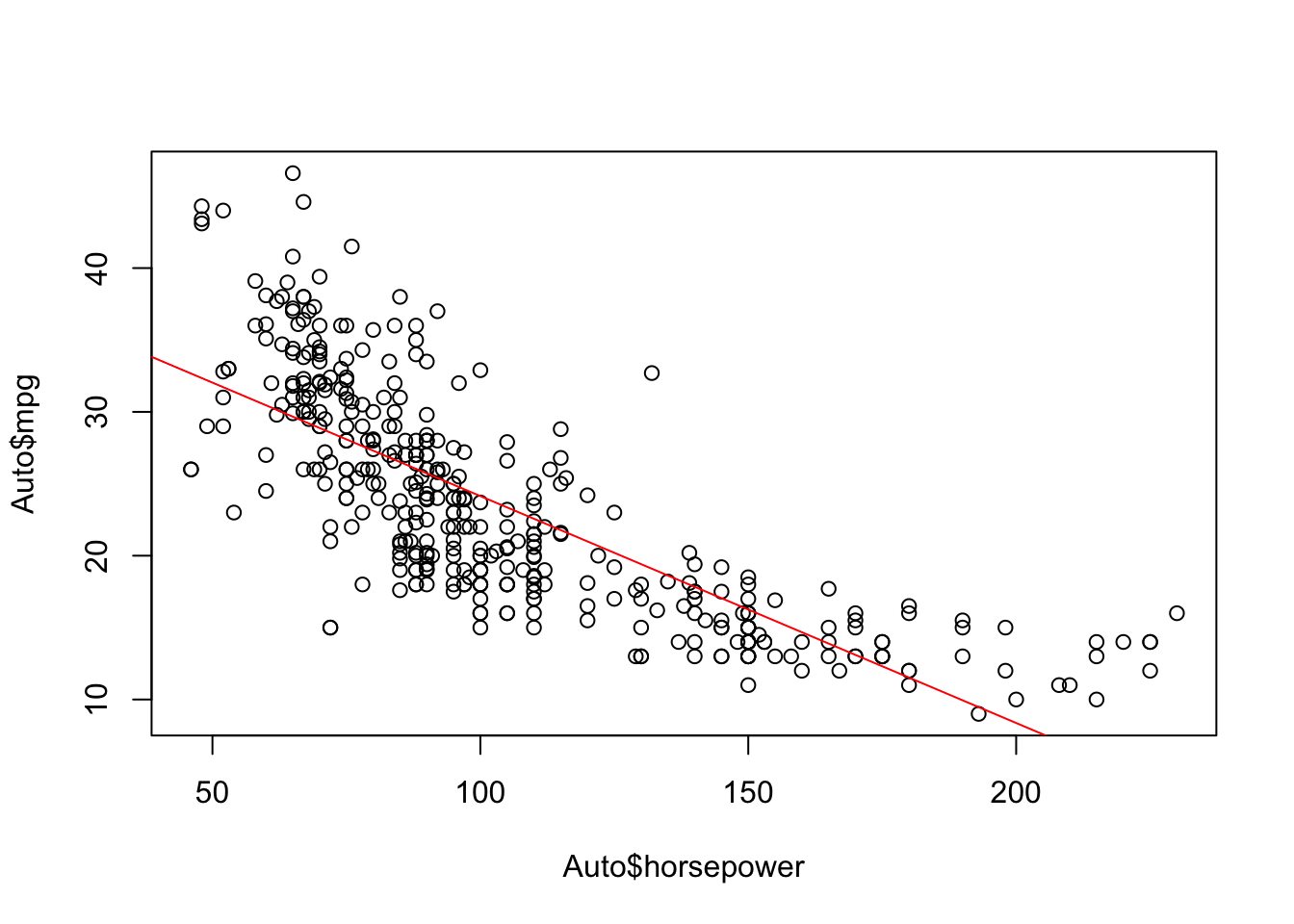
Use the plot() function to produce diagnostic plots of the least squares regression fit.
使用 plot() 函数生成最小二乘回归拟合的诊断图。

Comment on any problems you see with the fit.
对任何你认为适合的问题进行评论。

par(mfrow=c(2,2))

plot(fitlm)

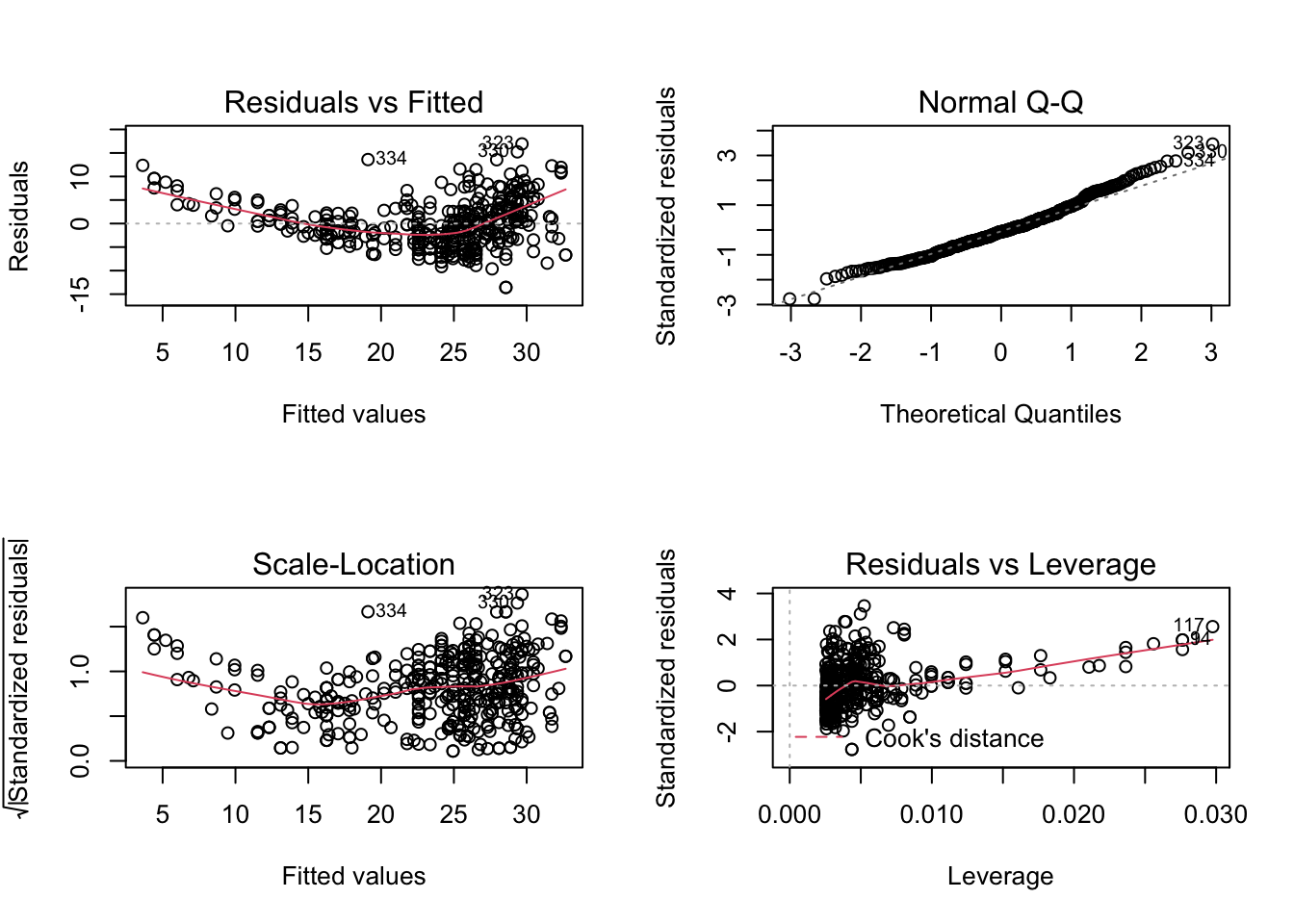
• residuals vs fitted plot shows that the relationship is non-linear
  残差与拟合图的关系是非线性的

# In-Class Exercise

Construct a simple linear regression of mpg with cylinders , displacement , and acceleration respectively.
分别用 cylinders “气缸”、 displacement “位移” 和 acceleration “加速度” 构建一个简单的 mpg 线性回归。

Based on the output, answer the following questions:
根据输出结果，回答以下问题:

• Is there a relationship between the predictor and the response?
  预测变量和响应变量之间有关系吗？

• How strong is the relationship between the predictor and the response?
  预测变量和响应变量之间的关系有多强？

• Is the relationship between the predictor and the response positive or negative?
  预测变量和响应变量之间的关系是积极的还是消极的？

• Based on the RSE and $R^2$, which model will you choose for the simple linear regression? Explain it.
  基于 RSE 和 $R^2$，你会选择哪个模型进行简单的线性回归？解释它。

# Reference

1. Chapter 3 of the textbook Gareth James, Daniela Witten, Trevor Hastie and Robert Tibshirani,
   An Introduction to Statistical Learning: with Applications in R.

2. Chapter 11 of the textbook Chantal D. Larose and Daniel T. Larose
   Data Science Using Python and R.

3. Part of this lecture notes are extracted from Prof. Sonja Petrovic ITMD/ITMS 514 lecture notes.