# Part ONE: Review the approach to location and scale problems for one and two populations

For inference on population mean, which of the following could we potentially use? Choose all apply
- The normal distribution (with the Z statistic)
- The t-distribution (with the T statistic)
- The chi-square distribution (with the $\chi^2$ statistic)
- The F-distribution (with the F statistic)
For inference on population mean when population variance is known, which of the following should we use? (In this part, suppose X_1, ... , X_1000 is a random sample (of size 1000) from some unknown distribution.)
- The normal distribution (with the Z statistic)
- The normal distribution (with the Z statistic), but ONLY if X comes from a normal distribution
- The t-distribution (with the T statistic)
- The t-distribution (with the T statistic), but ONLY if X comes from a normal distribution
For inference on population mean when population variance is unknown, which of the following should we use? (In this part, suppose X_1, ... , X_1000 is a random sample (of size 1000) from some unknown distribution.)
- The normal distribution (with the Z statistic)
- The normal distribution (with the Z statistic), but ONLY if X comes from a normal distribution
- The t-distribution (with the T statistic)
- The t-distribution (with the T statistic), but ONLY if X comes from a normal distribution
For inference on population variance, which of the following distributions will be useful?
- normal
- $T$
- $\chi^2$
- $F$
For comparing variances between two populations, which of the following distributions will be useful?
- normal
- $T$
- $\chi^2$
- $F$

# Part Two: Confidence Interval and Hypothesis Testing (35 points)

# Problem 1.

An electrical firm manufactures light bulbs that have a length of life that is approximately normally distributed, with mean equal to 800 hours and a standard deviation of 40 hours. A random sample of 16 bulbs will have an average life of less than 775 hours. (15 points)

a. Give a probabilistic result that indicates how rare an event $\bar{X} \leq 775$ is when $\mu= 800$ . On the other hand, how rare would it be if $\mu$ truly were, say, 760 hours?

By Central Limit Theory, we know when n is large,

$\frac{\bar{x}-\mu}{\sigma/\sqrt{n}} \sim \mathcal{N}(0,1) \Longrightarrow \bar{x} \sim \mathcal{N}(\mu,\sigma/\sqrt{n})$

	nsize <- 16 # Sample Size
	sigma <- 40/sqrt(nsize) # Sample standard deviation

	mu <- 800 # Sample mean
	p <- pnorm(775, mean = mu, sd = sigma)
	p

	mu <- 760 # if sample mean were 760
	p <- pnorm(775, mean = mu, sd = sigma)
	p

[1] 0.006209665
[1] 0.9331928

	# mu = 800, P(xbar<=775)
	pnormGC(775, mean =800, sd =40/sqrt(16), graph = TRUE)

[1] 0.006209665

	# mu = 760, P(xbar<=775)
	pnormGC(775, mean =760, sd =40/sqrt(16), graph = TRUE)

[1] 0.9331928

Conclusion: When $\mu = 800, P(\bar{X} \le 775) = 0.0062$ ; however, $\mu = 760, P(\bar{X} \le 775) = 0.9332$ . This tells us based on the sample that it is more likely $\mu$ should be 760 instead of 800.

b. Please construct a 95% confidence interval on $\mu$ with $\bar{X} = 775$ . Is 800 inside the interval?

	alpha <- 0.05
	zalpha2 <- qnorm(1-alpha/2)
	sd <- 40
	n <- 16
	xbar <- 775
	loBd <- xbar-zalpha2*sd/sqrt(n)
	loBd

[1] 755.4004

	upBd <- xbar+zalpha2*sd/sqrt(n)
	upBd

[1] 794.5996

Conclusion: 95% confidence interval is (755.4,794,6). 800 is not inside the interval.

c. We wish to test

$H_0: \mu = 800, \\ H_1: \mu \ne 800.$

Will you reject $H_0$ suppose $\bar{X}=775$ ? Justify your answer.

$Z=\frac{\bar{x}-\mu}{\sigma/\sqrt{n}}$ . We want to calculate zvalue first. If consider $\sigma$ = 0.05%, the reject region is $|z|> z_{0.025} = 1.96$

	z <- (xbar-800)/(sd/sqrt(n))
	z

[1] -2.5

	#pvalue
	2*pnormGC(z)

[1] 0.01241933

We can find $z<-z_{0.025}$ and p-value < 0.05, therefore, we should reject $H_0$ .

# Problem 2.

A maker of a certain brand of low-fat cereal bars claims that the average saturated fat content is 0.5
gram. In a random sample of 8 cereal bars of this brand, the saturated fat content was 0.6, 0.7, 0.7, 0.3, 0.4, 0.5, 0.4, and 0.2. Assume a normal distribution. (10 points)

Please construct a 95% confidence interval on the average saturated fat content.
Would you agree with the claim? Justify your answer.

We consider using t-test, as we don’t know the variance.

	fat <-c(0.6, 0.7, 0.7, 0.3, 0.4, 0.5, 0.4, 0.2)
	t.test(fat,alternative = c("two.sided"), mu = 0.5, conf.level = 0.95)

    One Sample t-test

data:  fat
t = -0.38592, df = 7, p-value = 0.711
alternative hypothesis: true mean is not equal to 0.5
95 percent confidence interval:
 0.32182 0.62818
sample estimates:
mean of x 
    0.475

Base on the results, we find the 95% confidence interval is (0.32182,0.62818) and p value is much larger than 0.05. We should not reject $H_0$ .

# Problem 3. Checking out some small data sets that come with R (10 points)

In this problem, you will load and work with the mtcars data set in R.

Two data samples are independent if they come from unrelated populations and the samples does not affect each other. Here, we assume that the data populations follow the normal distribution.

In the data frame column mpg (which stands for "miles per galon") of the data set mtcars , there are gas mileage data of various 1974 U.S. automobiles. Let's take a look:

mtcars$mpg

 [1] 21.0 21.0 22.8 21.4 18.7 18.1 14.3 24.4 22.8 19.2 17.8 16.4 17.3 15.2 10.4
[16] 10.4 14.7 32.4 30.4 33.9 21.5 15.5 15.2 13.3 19.2 27.3 26.0 30.4 15.8 19.7
[31] 15.0 21.4

Meanwhile, another data column in mtcars , named am , indicates the transmission type of the automobile model (0 = automatic, 1 = manual):

mtcars$am

 [1] 1 1 1 0 0 0 0 0 0 0 0 0 0 0 0 0 0 1 1 1 0 0 0 0 0 1 1 1 1 1 1 1

In particular, the gas mileage for manual and automatic transmissions are two independent data populations.

Assume that the data in mtcars follows the normal distribution, let us look for whether the difference between the mean gas mileage of manual and automatic transmissions seems to be statistically significant.

Hints and shortcuts The gas mileage for automatic transmission can be listed as follows:

	L = mtcars$am == 0
	mpgAuto = mtcars[L,]$mpg
	mpgAuto # automatic transmission mileage

 [1] 21.4 18.7 18.1 14.3 24.4 22.8 19.2 17.8 16.4 17.3 15.2 10.4 10.4 14.7 21.5
[16] 15.5 15.2 13.3 19.2

By applying the negation of L, we can find the gas mileage for manual transmission:

	mpgManual = mtcars[!L,]$mpg
	mpgManual # manual transmission mileage

 [1] 21.0 21.0 22.8 32.4 30.4 33.9 27.3 26.0 30.4 15.8 19.7 15.0 21.4

a. Please construct a hypothesis test for ratio of the variances of these two populations. Then choose the appropriate test to make a conclusion.

The hypothesis testing should be

$H_0:\sigma^2_{auto}/\sigma^2_{manual} = 1, \\ H_1:\sigma^2_{auto}/\sigma^2_{manual} \ne 1$

	# alpha = 0.05
	var.test(mpgAuto,mpgManual,alternative = c("two.sided"),conf.level = 0.95)

    F test to compare two variances

data:  mpgAuto and mpgManual
F = 0.38656, num df = 18, denom df = 12, p-value = 0.06691
alternative hypothesis: true ratio of variances is not equal to 1
95 percent confidence interval:
 0.1243721 1.0703429
sample estimates:
ratio of variances 
         0.3865615

	# alpha = 0.1
	var.test(mpgAuto,mpgManual,alternative = c("two.sided"),conf.level = 0.9)

    F test to compare two variances

data:  mpgAuto and mpgManual
F = 0.38656, num df = 18, denom df = 12, p-value = 0.06691
alternative hypothesis: true ratio of variances is not equal to 1
90 percent confidence interval:
 0.1505051 0.9053528
sample estimates:
ratio of variances 
         0.3865615

If we consider $\alpha = 0.05$ , we can not reject $H_0$ . However, if $\alpha = 0.1$ , based on the result, we should consider to reject $H_0$ .

b. Based on the result in a), construct a hypothesis test for the means of these two populations. Show your conclusion.

The hypotheis test is

$H_0: \mu_{auto}-\mu_{manual} = 0, \\ H_1: \mu_{auto}-\mu_{manual} \ne 0$

If we consider $\alpha = 0.05$ , we have the variances are the same. Thus we use the condition variances are equal but unknown.

t.test(mpgAuto,mpgManual,alternative = c("two.sided"), var.equal = TRUE, conf.level = 0.95)

    Two Sample t-test

data:  mpgAuto and mpgManual
t = -4.1061, df = 30, p-value = 0.000285
alternative hypothesis: true difference in means is not equal to 0
95 percent confidence interval:
 -10.84837  -3.64151
sample estimates:
mean of x mean of y 
 17.14737  24.39231

However, if we choose $\alpha = 0.1$ , we should use the condition variances are not equal.

t.test(mpgAuto,mpgManual,alternative = c("two.sided"), var.equal = FALSE, conf.level = 0.9)

    Welch Two Sample t-test

data:  mpgAuto and mpgManual
t = -3.7671, df = 18.332, p-value = 0.001374
alternative hypothesis: true difference in means is not equal to 0
90 percent confidence interval:
 -10.576623  -3.913256
sample estimates:
mean of x mean of y 
 17.14737  24.39231

No matter what value of $\alpha$ , based on the result, we should reject $H_0$ .

# Part Three: Working With Data (50 points)

# Instructions: Please review EDA Handout first. Import the needed packages first.

Obtaining the adult dataset

# Tasks

For the following exercises, work with the adult.data data set. Use either Python or R to solve each
problem. Please read the adult.name file to understand each attribute.

a. Import the adult.data data set and name it adult . (5 points)

	adult <- read.csv("adult.data", header=FALSE)
	# View(adult)

To make the plot better, we rename all the attributes.

names(adult)[1:15] <- c("age","workclass", "fnlwgt", "education","education-num","marital-status","occupation","relationship","race","sex","capital-gain","capital-loss","hours-per-week","native-country","class(response)")

b. Standardize hours-per-week and indicate if there is any outlier (5 points)

	hrsWeek_z <- scale(adult$`hours-per-week`)
	adult_outliers <- adult[hrsWeek_z < -3\| hrsWeek_z>3,]
	#too many outliers, just show the first six records
	head(adult_outliers)

    age         workclass fnlwgt     education education-num
11   37           Private 280464  Some-college            10
29   39           Private 367260       HS-grad             9
78   67                 ? 212759          10th             6
158  71  Self-emp-not-inc 494223  Some-college            10
190  58         State-gov 109567     Doctorate            16
273  50  Self-emp-not-inc  30653       Masters            14
         marital-status       occupation   relationship   race   sex
11   Married-civ-spouse  Exec-managerial        Husband  Black  Male
29             Divorced  Exec-managerial  Not-in-family  White  Male
78   Married-civ-spouse                ?        Husband  White  Male
158           Separated            Sales      Unmarried  Black  Male
190  Married-civ-spouse   Prof-specialty        Husband  White  Male
273  Married-civ-spouse  Farming-fishing        Husband  White  Male
    capital-gain capital-loss hours-per-week native-country class(response)
11             0            0             80  United-States            >50K
29             0            0             80  United-States           <=50K
78             0            0              2  United-States           <=50K
158            0         1816              2  United-States           <=50K
190            0            0              1  United-States            >50K
273         2407            0             98  United-States           <=50K

boxplot(adult$`hours-per-week`)

Answer: Based the two methods, we can find there are a lot of outliers of hours-per-week .

c. Show a bar graph of race with a response class overlay. What conclusion can you draw from the bar graph? (10 points)

table(adult$race,adult$`class(response)`)

                       <=50K  >50K
   Amer-Indian-Eskimo    275    36
   Asian-Pac-Islander    763   276
   Black                2737   387
   Other                 246    25
   White               20699  7117

	ggplot(data = adult,mapping = aes(x =race, fill = `class(response)`)) +
	geom_bar()

	ggplot(data = adult,mapping = aes(x =race, fill = `class(response)`))+
	geom_bar(position = "fill")

If we don’t use fill , we can find White is dominated in the race attribute. If we want to compare the percentage of >50k in each category, we should use fill . The interesting thing is the percentage of >50k in Asian-Pac-Islander are competitive to the percentage in White . The other category actally has the lowest percentage.

d. Select any numeric attribute and show a histogram of it with a response class overlay. What conclusion can you draw from the histogram? (10 points)

I choose hours-per-week as the attribute.

ggplot(data = adult,mapping = aes(x =`hours-per-week`, fill = `class(response)`)) + geom_histogram(binwidth = 10)

ggplot(data = adult,mapping = aes(x =`hours-per-week`, fill = `class(response)`)) + geom_histogram(binwidth = 10, color = "black",position = "fill")

Here I use the binwidth is 10. If you choose different options, the graph will be slightly different and the tendency will be the same. If we don’t use fill , it is easy to know working hours around 40 should dominate in hours-per-week and about 25% in the class of >50k . However, the highest percentage of >50k occurs at the working hours from 45 to 65 instead of the 40 bin. Someone can get >50k income when they almost don’t work.

e. Select any two attributes and show a plot, what conclusion can you draw from the plot? (10 points)

Here, I choose sex and class as two attributes.

	ggplot(data = adult, mapping = aes(x = `sex`,fill = `class(response)`)) +
	geom_bar()

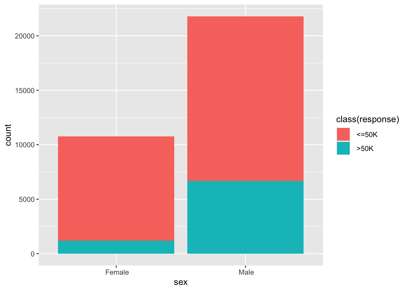
	ggplot(data = adult, mapping = aes(x = `sex`,fill = `class(response)`)) +
	geom_bar(position = 'fill')

In this dataset, the number of male is almost double of the number of female. More than that, the percentage of >50k for male is almost triple of the percentage for female.

f. Select any three attributes and plot their relationship using 2D scatter plot, use one of the selected attributes as the color code when plotting, what can you say about the correlation of these attributes? What conclusion can you draw from the plot? (10 points)

Here, I choose age , hours=per-week , and class as the attributes.

	ggplot(data = adult) +
	geom_point(mapping = aes(x = age, y = `hours-per-week`,colour = `class(response)`))

If your age is less than 25, even you work 100 hrs per week, it is still difficult for you to make income >50k . When you are older than 75, it is not easy for you to make >50k . The income is not proportional to the work-per-hours .

# Extra Points (10 points)

One claim "Female and Male have the same proportion >50k of the class ". Can you use what you learn in class to reject or fail to reject the statement? Justify your answer.

Hint: Need a proportion test here.

$H_0: p_{female} = p_{male}, \\ H_1: p_{female} \ne p_{male}.$

	sexresponsetable<-table(adult$sex,adult$`class(response)`)
	x11 <- sexresponsetable[1,1]
	x12 <- sexresponsetable[1,2]
	x21 <- sexresponsetable[2,1]
	x22 <- sexresponsetable[2,2]
	prop.test(x = c(x12,x22),n = c(x11+x12,x21+x22),conf.level = 0.95)

    2-sample test for equality of proportions with continuity correction

data:  c out of cx12 out of x11 + x12x22 out of x21 + x22
X-squared = 1517.8, df = 1, p-value < 2.2e-16
alternative hypothesis: two.sided
95 percent confidence interval:
 -0.2048416 -0.1877104
sample estimates:
   prop 1    prop 2 
0.1094606 0.3057366

Based on the result, p-value is much smaller than 0.05, we should reject $H_0$ . Female and Male do NOT have the same proportion >50k of the class

How to solve using z-test?

	p1hat <- x12/(x11+x12)
	p2hat <- x22/(x21+x22)
	phat <- (x12+x22)/(x11+x12+x21+x22)
	#get z statistic
	zvalue <- (p1hat-p2hat)/(sqrt(phat(1-phat)(1/(x11+x12)+1/(x21+x22))))
	zvalue

[1] -38.9729

	#get critical region
	alpha <- 0.05
	zalpha <- qnorm(1-alpha)
	zalpha

[1] 1.644854

	#get p-value
	pnorm(zvalue) #why?

[1] 0

p-value is close to 0, we should reject $H_0$ .