# Objectives 目标
- Understand Bernoulli Distribution and Binoimal Distribution
了解伯努利分布和二项分布
Bernoulli and Binomial distributions are related to experiments with binary outcomes (success or failure).
伯努利分布和二项分布与二元结果(成功或失败)的实验有关。 - Understand the interpretation of these distributions
理解这些分布的解释 - Know how to do the simulations of these two experiments and
barplot
知道如何做这两个实验的模拟和barplot - Know how to use
sampleto generate training and testing data set
知道如何使用sample生成训练和测试数据集
# Bernoulli Distribution 伯努利分布
- Bernoulli Experiment 伯努利实验
- A single random experiment with outcome either success or failure, and the probability of the success is .
一个随机实验,结果要么成功要么失败,成功的概率是 。
Examples: Flip a single coin; Attempt a free throw
例子: 抛一枚硬币;尝试罚球 - Bernoulli Random Variable 伯努利随机变量
- A random variable that takes either or , where it takes 1 when the outcome of the Bernoulli trial is a success and 0 when the outcome of the Bernoulli trial is a failure.
一个随机变量 或者 ,当伯努利试验的结果成功时取 1,当伯努利试验的结果失败时取 0。 - Bernoulli Distribution 伯努利分布
- The distribution of a Bernoulli random variable is called the Bernoulli distribution.
伯努利随机变量的分布称为伯努利分布。
- Probability Mass Function of Bernoulli Distribution/Random Variable:
伯努利分布 / 随机变量的概率质量函数:
| 0 | 1 | |
- Expectation and Variance 期望值和方差值
# A Simple Example: We toss a fair coin. 扔一枚公平的硬币
Each time of the tossing coin is a Bernoulli Experiment. Consider head is success (1).
每次抛硬币都是伯努利实验。考虑头像面是成功(1)。What is the probability ?
概率 是多少?n <- 10 # number of random experiments
x <- c(0,1) # sample space for tossing a coin, 0--Tail, 1--Head
coinToss <- sample(x, size=n, replace=TRUE)
# generate n outcomes of the experimentsmean(coinToss)
[1] 0.4What about 100 times? 100 次呢?
n <- 100 # number of random experiments
x <- c(0,1) # sample space for tossing a coin, 0--Tail, 1--Head
coinToss <- sample(x, size=n, replace=TRUE)
# generate n outcomes of the experimentsmean(coinToss)
[1] 0.5Seems close to . Let's try .
似乎接近 了,再试试 。n <- 1000000 # number of random experiments
x <- c(0,1) # sample space for tossing a coin, 0--Tail, 1--Head
coinToss <- sample(x, size=n, replace=TRUE)
# generate n outcomes of the experimentsmean(coinToss)
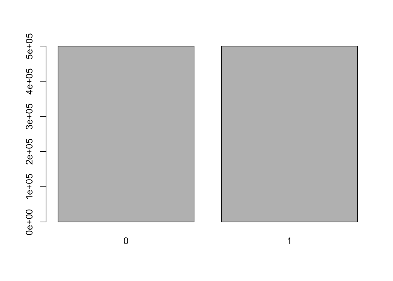
[1] 0.5We can use a
barplotto generate the frequence forcoinToss
我们可以使用abarplot来生成频率coinTossbarplot(table(coinToss)) #
![]()
# the sample function is also used to split a data set
sample 函数还用于拆分数据集
例如机器学习数据挖掘部分,将考虑 80% 作为训练数据,20% 作为测试数据。
i <- sample(2, nrow(cars), replace=TRUE, prob=c(0.8, 0.2)) # prob 后面跟着的是两个概率 | |
carsTrainingData <- cars[i==1,] # 等于 1 的数据归于训练集 | |
carsTestingData <- cars[i==2,] # 等于 2 的数据归于测试集 | |
summary(cars) |
    speed           dist
Min.   : 4.0   Min.   :  2.00
1st Qu.:12.0   1st Qu.: 26.00
Median :15.0   Median : 36.00
Mean   :15.4   Mean   : 42.98
3rd Qu.:19.0   3rd Qu.: 56.00
Max.   :25.0   Max.   :120.00
summary(carsTrainingData) |
    speed            dist
Min.   : 4.00   Min.   :  2.0
1st Qu.:12.00   1st Qu.: 26.0
Median :15.00   Median : 35.0
Mean   :15.19   Mean   : 41.9
3rd Qu.:18.75   3rd Qu.: 54.0
Max.   :24.00   Max.   :120.0
summary(carsTestingData) |
    speed           dist
Min.   : 7.0   Min.   :16.00
1st Qu.:11.0   1st Qu.:23.50
Median :18.0   Median :52.00
Mean   :16.5   Mean   :48.62
3rd Qu.:21.0   3rd Qu.:68.50
Max.   :25.0   Max.   :85.00
# In-class Exercise
Please use the above the code to divide the
irisdata set into two parts, in training data set and in testing data set请使用上面的代码将
iris数据集分成两部分, 在训练数据集和 在测试数据集iris i <- sample(2, nrow(iris), replace=TRUE, prob=c(0.8, 0.2)) # prob 后面跟着的是两个概率
irisTrainingData <- iris[i==1,] # 等于 1 的数据归于训练集
irisTestingData <- iris[i==2,] # 等于 2 的数据归于测试集
summary(iris)
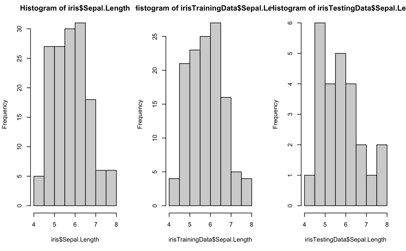
 Sepal.Length    Sepal.Width     Petal.Length    Petal.Width          Species
Min.   :4.300   Min.   :2.000   Min.   :1.000   Min.   :0.100   setosa    :50
1st Qu.:5.100   1st Qu.:2.800   1st Qu.:1.600   1st Qu.:0.300   versicolor:50
Median :5.800   Median :3.000   Median :4.350   Median :1.300   virginica :50
Mean   :5.843   Mean   :3.057   Mean   :3.758   Mean   :1.199
3rd Qu.:6.400   3rd Qu.:3.300   3rd Qu.:5.100   3rd Qu.:1.800
Max.   :7.900   Max.   :4.400   Max.   :6.900   Max.   :2.500
Do some data exploration in these two data sets. E.g.
summary,histogram,boxplot, orbarplot在这两个数据集中做一些数据探索。
summary(irisTrainingData)
Sepal.Length Sepal.Width Petal.Length Petal.Width Species Min. :4.300 Min. :2.000 Min. :1.000 Min. :0.100 setosa :40 1st Qu.:5.100 1st Qu.:2.800 1st Qu.:1.600 1st Qu.:0.300 versicolor:44 Median :5.800 Median :3.000 Median :4.400 Median :1.400 virginica :41 Mean :5.853 Mean :3.074 Mean :3.783 Mean :1.217 3rd Qu.:6.400 3rd Qu.:3.400 3rd Qu.:5.100 3rd Qu.:1.800 Max. :7.900 Max. :4.400 Max. :6.900 Max. :2.500summary(irisTestingData)
Sepal.Length Sepal.Width Petal.Length Petal.Width Species Min. :4.400 Min. :2.200 Min. :1.200 Min. :0.200 setosa :10 1st Qu.:5.000 1st Qu.:2.600 1st Qu.:1.500 1st Qu.:0.200 versicolor: 6 Median :5.700 Median :3.000 Median :4.000 Median :1.300 virginica : 9 Mean :5.796 Mean :2.976 Mean :3.632 Mean :1.112 3rd Qu.:6.300 3rd Qu.:3.200 3rd Qu.:5.200 3rd Qu.:1.800 Max. :7.700 Max. :3.900 Max. :6.700 Max. :2.300par(mfrow=c(1,3))
hist(iris$Sepal.Length)
hist(irisTrainingData$Sepal.Length)
hist(irisTestingData$Sepal.Length)
![]()
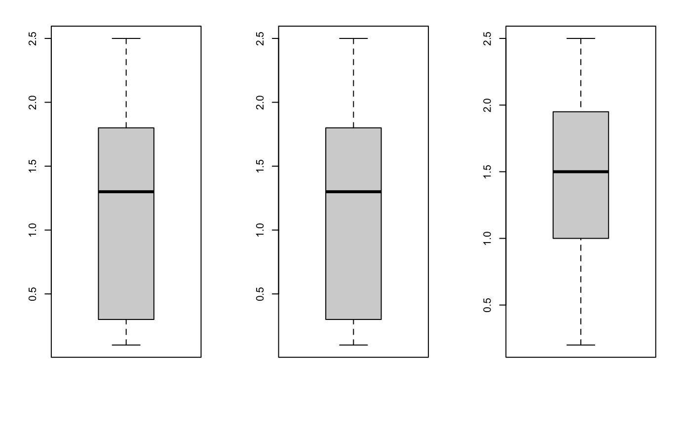
par(mfrow=c(1,3))
boxplot(iris$Petal.Width)
boxplot(irisTrainingData$Petal.Width)
boxplot(irisTestingData$Petal.Width)
![]()
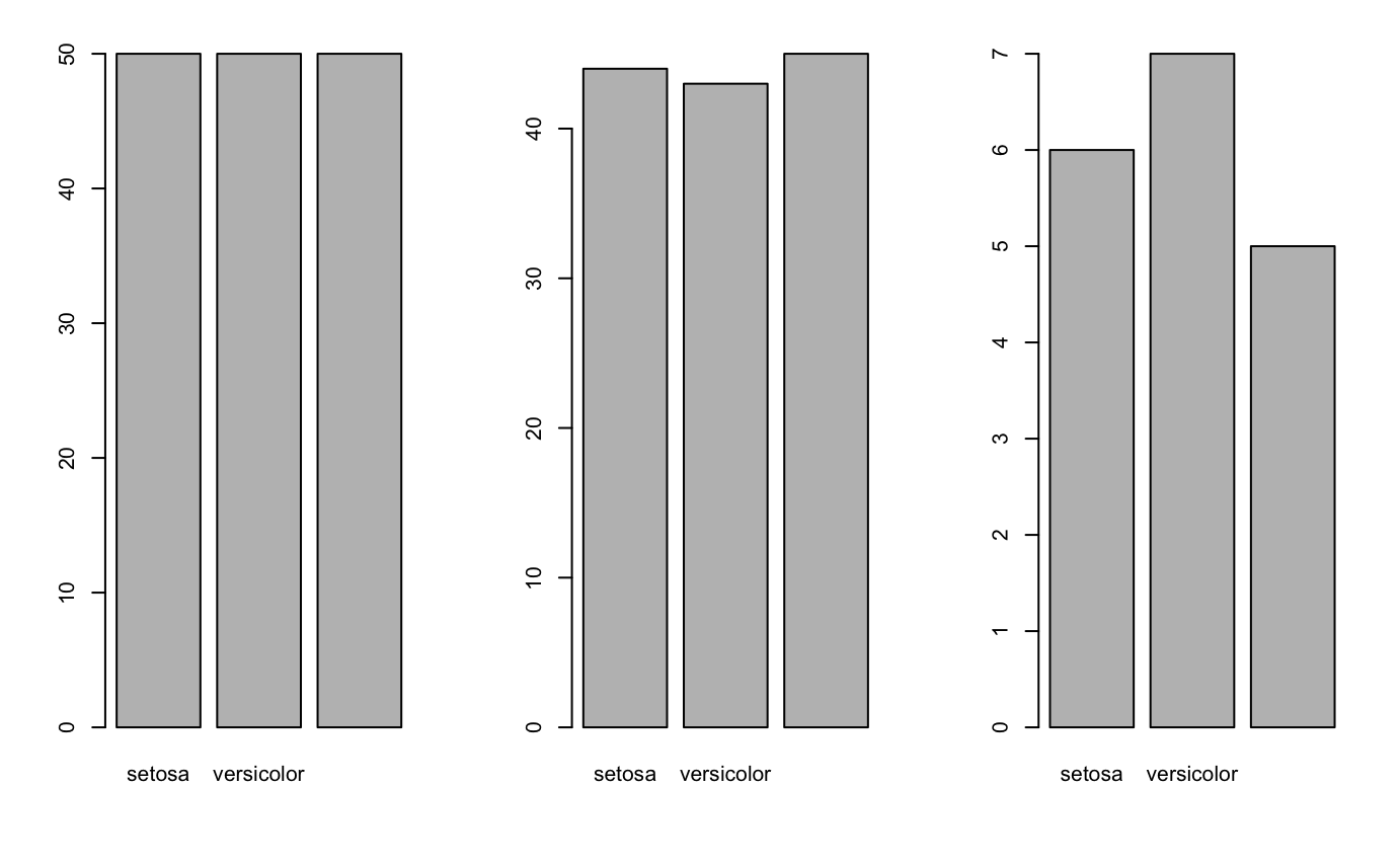
par(mfrow=c(1,3))
barplot(table(iris$Species))
barplot(table(irisTrainingData$Species))
barplot(table(irisTestingData$Species))
![]()
# If we have an unfair coin 如果扔一个不公平的硬币
what should we do? 我们应该怎么做?
Suppose we have one unfair coin, whose probabilities of heads are .
假设我们有一枚不公平的硬币,其正面概率为.How many heads will we get, if we flip the coin 10 times? 100 times? 1000 times?
如果我们抛硬币 10 次,我们会得到多少个正面?抛 100 次?抛 1000 次?unfaircoin p = 0.25;
n = 10;
x = c(0,1)
unfairCoinToss <- sample(x, size=n, replace=TRUE, prob = c(1-p,p))
sum(unfairCoinToss)
[1] 2n = 100;
unfairCoinToss <- sample(x, size=n, replace=TRUE, prob = c(1-p,p))
sum(unfairCoinToss)
[1] 30n = 1000;
unfairCoinToss <- sample(x, size=n, replace=TRUE, prob = c(1-p,p))
sum(unfairCoinToss)
[1] 241Question: Do these results make sense?
问题:这些结果有意义吗?
# In-class Exercise
Suppose I have an unfair coin, whose probabilities of heads are . Can you modify the code above to find the number of heads when flipping the code times?
假设我有一枚不公平的硬币,其正面概率为 . 能不能修改上面的代码,求抛 次正面朝上的次数?
p = 0.6
n = 1e6
x = c(0, 1)
unfairCoinToss <- sample(x, size=n, replace=TRUE, prob = c(1-p,p))
sum(unfairCoinToss)
# Binomial Distribution 二项分布
- Binomial Experiment 二项式实验
- Repeat Bernoulli experiment independently for a certain number () of times, each repetition has the same possible outcomes (success or failure), and the probability of each success () is consistent for all trials. This experiment is called Binomial trial.
独立重复伯努利实验一定数量() 次,每次重复都有相同的可能结果(成功或失败),以及每次成功的概率() 对于所有试验都是一致的。这个实验叫做二项式试验。 - Binomial Random Variable 二项式随机变量
- The number of of a binomial experiment is called a Binomial random variable.
二项式实验结果的发生次数 X 称为二项式随机变量。 - Binomial Distribution 二项式分布
- The distribution of a Binomial random variable is called the binomial distribution
二项式随机变量的分布称为二项式分布
# Examples: Number of heads in 40 coin flips, Number of hits in 20 free throws
示例:40 次抛硬币的正面次数,20 次罚球的命中次数
PMF: ,
Expectation and Variance 期望值和方差值
Let denote the Bernoulli random variable.
表示伯努利随机变量。This is becasue are independent and identical distributed (iid).
这是因为 是独立同分布的(iid)。
# Another Simple Example: We toss a fair coin 扔一枚公平的硬币
Each time of the tossing coin is a Bernoulli Experiment. Consider head is success (1).
每次抛硬币都是伯努利实验。考虑头像面是成功(1)。Suppose we toss this coin 10 times, how many heads can we get?
假设我们抛这枚硬币 10 次,我们能得到几个正面?n <- 10 # number of random experiments
x <- c(0,1) # sample space for tossing a coin, 0--Tail, 1--Head
coinToss <- sample(x, size=n, replace=TRUE)
# generate n outcomes of the experimentssum(coinToss)
[1] 61000000 times?
n <- 10000000 # number of random experiments
x <- c(0,1) # sample space for tossing a coin, 0--Tail, 1--Head
coinToss <- sample(x, size=n, replace=TRUE)
# generate n outcomes of the experimentssum(coinToss)
[1] 5001636Let's explore how this value varies in repeated experiments.
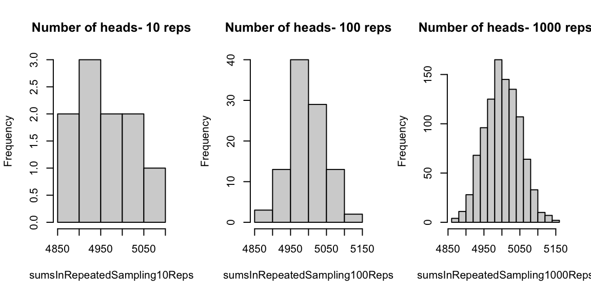
这个值在重复实验中是如何变化的distrib-of-heads n <- 10000
x <- c(0,1)
sumsInRepeatedSampling10Reps<-replicate(10, sum(sample(x, size=n, replace=TRUE)))
sumsInRepeatedSampling100Reps<-replicate(100, sum(sample(x, size=n, replace=TRUE)))
sumsInRepeatedSampling1000Reps<-replicate(1000, sum(sample(x, size=n, replace=TRUE)))
par(mfrow=c(1,3))
hist(sumsInRepeatedSampling10Reps,main = paste("Number of heads- 10 reps"))
hist(sumsInRepeatedSampling100Reps,main = paste("Number of heads- 100 reps"))
hist(sumsInRepeatedSampling1000Reps,main = paste("Number of heads- 1000 reps"))
![]()
# Conclusions 结论
The number of heads observed--we know it is --when tossing a coin times is a statistics computed from the sample of coin tosses.
头像面数 ,抛硬币 次是从抛 次硬币样本计算的统计数据。
should follow the Binomial distribution.
应该服从二项分布
The experiments above suggest that the sampling distribution of appears to have a mean around the expected number of heads when a fair coin is tossed, which is about or .
上述实验表明,抽样分布 当抛一枚公平的硬币时,似乎在预期的正面次数附近有一个平均值,大约是 或者。
The more times we repeat the experiment of coin tosses, the closer gets to its expected value -- this can be measured by looking at both the mean and the variance of
我们重复掷硬币的实验次数 越多, 离其预期值越近 —— 这可以通过查看 的均值和方差来衡量
meansOfX<-c(mean(sumsInRepeatedSampling10Reps), | |
mean(sumsInRepeatedSampling100Reps), | |
mean(sumsInRepeatedSampling1000Reps)) | |
varsOfX<-c(var(sumsInRepeatedSampling10Reps),var(sumsInRepeatedSampling100Reps),var(sumsInRepeatedSampling1000Reps)) | |
meansOfX |
[1] 4967.200 4993.110 5001.822
varsOfX |
[1] 3494.400 2393.452 2355.378
Question: is it possible that something similar to this always happens?
问题:是否有可能总是发生类似的事情?
As we will see, the sampling distribution of is approximately normal with mean equal to the expected value of . In other words, the example above illustrates a known result--the Central Limit Theorem, one of the cornerstone results used in inference!
正如我们将看到的,抽样分布 近似正态,均值等于期望值。 换句话说,上面的例子说明了一个已知的结果 —— 中心极限定理,这是推理中使用的基石结果之一!
# In-class Exercise: Roll A Die
Suppose we have a fair die. Modify the code above to simulate rolling a die 10 times, 1000 times, and 100000 times.
假设我们有一个公平的骰子。修改上面的代码来模拟掷骰子 10 次、1000 次和 100000 次。
10 times n <- 10
x <- 1:6
dieRoll <- sample(x, size=n, replace=TRUE)
barplot(table(dieRoll))
mean(dieRoll)
n <- 1000
dieRoll <- sample(x, size=n, replace=TRUE)
barplot(table(dieRoll))
mean(dieRoll)
n <- 100000
dieRoll <- sample(x, size=n, replace=TRUE)
barplot(table(dieRoll))
mean(dieRoll)
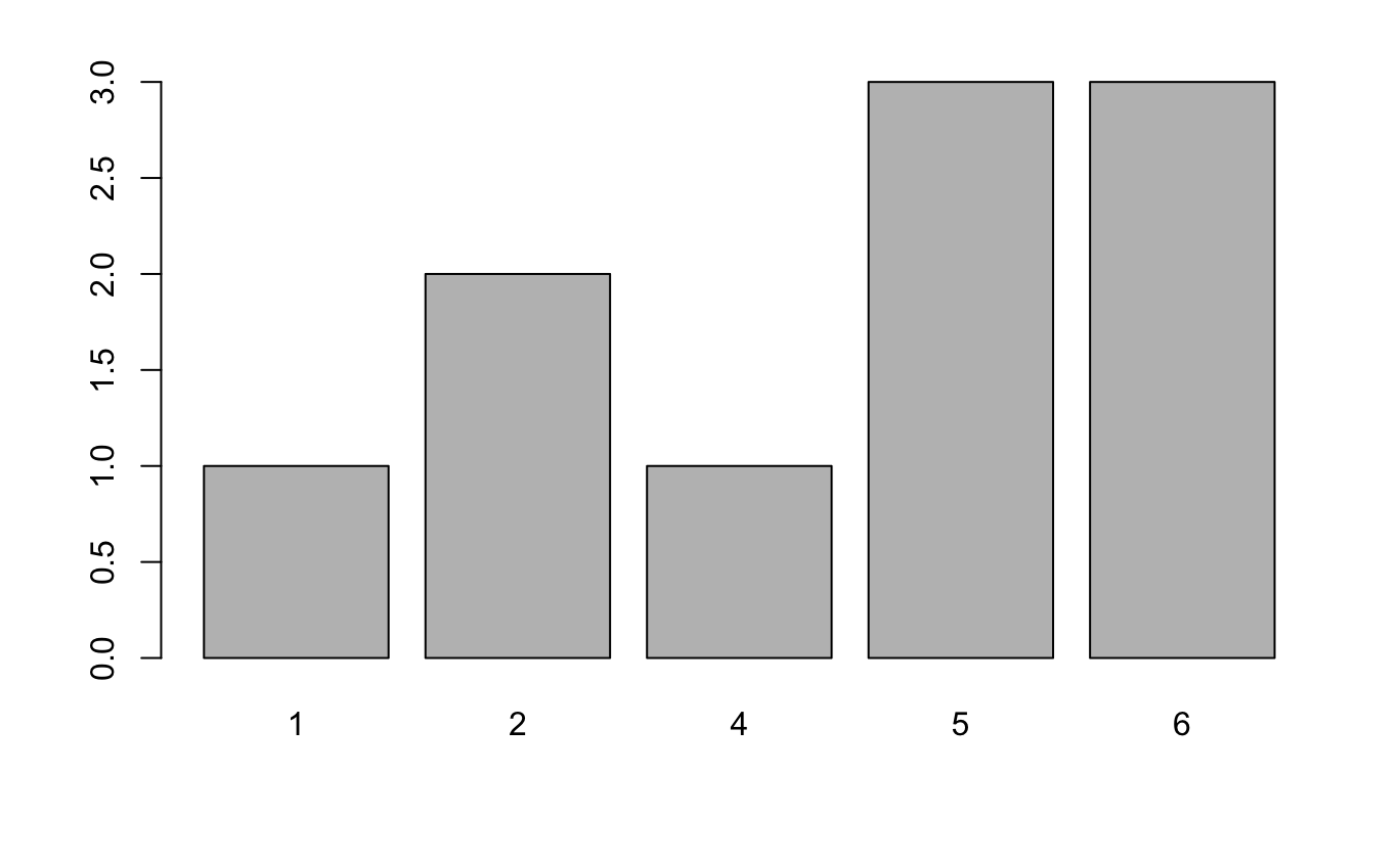
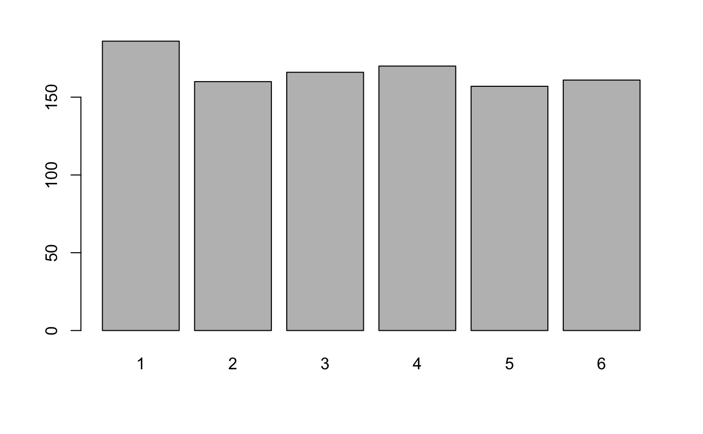
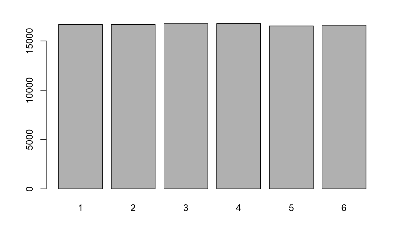
Do a barplot of the results in 1
对 1 中的结果进行条形图
![]()
![]()
![]()
Calculate the mean of the results in 1.
计算 1 中结果的平均值。
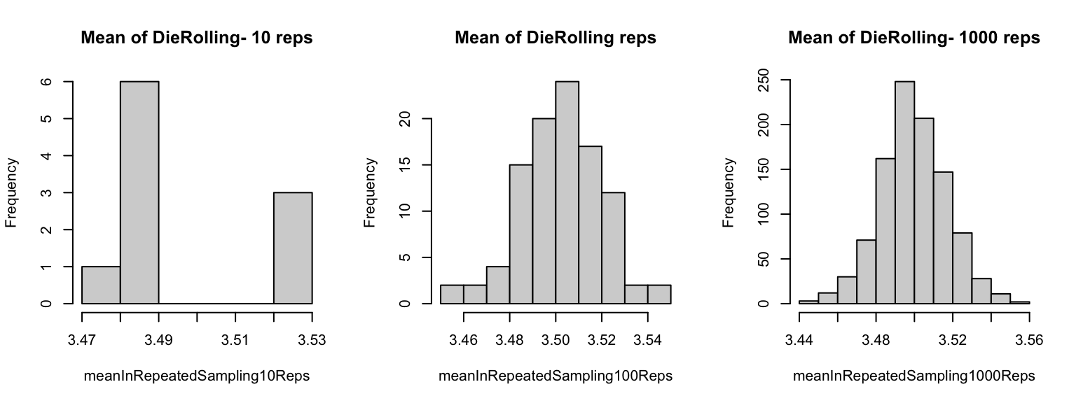
[1] 4.2
[1] 3.435
[1] 3.49603
Set to calculate the mean value. Then repeat your similuation 10, 100, and 1000 times. Save the results and do a histogram.
设定 计算平均值。然后重复模拟 10、100 和 1000 次。保存结果并绘制直方图。
n <- 10000
x = 1:6;
meanInRepeatedSampling10Reps<-replicate(10, mean(sample(x, size=n, replace=TRUE)))
meanInRepeatedSampling100Reps<-replicate(100, mean(sample(x, size=n, replace=TRUE)))
meanInRepeatedSampling1000Reps<-replicate(1000, mean(sample(x, size=n, replace=TRUE)))
par(mfrow=c(1,3))
hist(meanInRepeatedSampling10Reps,main = paste("Mean of DieRolling- 10 reps"))
hist(meanInRepeatedSampling100Reps,main = paste("Mean of DieRolling reps"))
hist(meanInRepeatedSampling1000Reps,main = paste("Mean of DieRolling- 1000 reps"))
![]()
One chanllenge question: Suppose this die is unfair. We can get number 1,3, and 5 with probability and 2, 4, and 6 with probability . How can we do the similar experiments as the in-class exercise?
假设这个骰子是不公平的。我们可以以 概率得到数字 1、3 和 5, 的概率得到 2、4 和 6。 我们如何做类似的实验?