# Overview 概述
Statistics (e.g. sample mean, sample variance, etc) are functions of random variables and therefore are also random variables themselves.
统计量(例如样本均值、样本方差等)是随机变量的函数,因此本身也是随机变量。
The distributions of the these statistics are called sampling distributions.
这些统计量的分布称为抽样分布。
Our inferred knowledge about these distributions is used to estimate parameters of the model which we postulate was used to generate the data.
对这些分布的推断知识,用来估算生成这些数据的假设模型的参数。
So far we have learned about point estimators and interval estimators.
我们到目前为止,我们已经了解了点估计和区间估计。
And now, we focus on hypothesis tests.
现在开始学习假设检验。
# Objectives 目标
- Understand what is hypothesis tests and -values
了解什么是假设检验和 值。 - Know how to choose the appropriate test for a hypothesis test
知道如何为假设检验选择合适的检验 - know how to interpret the result of a hypothesis test
知道如何解释假设检验的结果
# Overview of hypothesis testing 假设检验概述
A statistical hypothesis is an assertion or conjecture concerning one or more populations.
一个统计假设是关于一个断言或猜想的一个或多个总体。
For example, suppose that the hypothesis postulated by the engineer is that the fraction defective in a certain process is 0.10.
例如,工程师提出的假设是在特定过程中缺陷比例 是 0.10。
The experiment is to observe a random sample of the product in question.
实验是观察有关产品的随机样本。
Suppose that 100 items are tested and 12 items are found defective.
假设测试了 100 个项目,发现 12 个项目有缺陷。
It is reasonable to conclude that this evidence does not refute the condition that the binomial parameter and thus it may lead one not to reject the hypothesis.
可以合理地得出结论,该证据不能反驳二项式参数 的条件,因此它可能导致人们不拒绝这一假设。
However, it also does not refute or perhaps even
然而,它也不反驳 或者甚至 。
Rejection of a hypothesis implies that the sample evidence refutes it.
拒绝假设意味着样本证据驳斥了它。
Or, rejection means that there is a small probability of obtaining the sample information observed when, in fact, the hypothesis is true.
或者,拒绝意味着当实际上假设为真时,能观察到的样本信息的概率很小。
For example, for our proportion-defective hypothesis, a sample of 100 revealing 20 defective items is certainly evidence for rejection.
例如,对于我们的缺陷比例假设,100 个样本里显示 20 个缺陷项目则肯定是拒绝的证据。
Why? If, indeed, , the probability of obtaining 20 or more defectives is approximately .
为什么?如果 ,获得 20 个或更多次品的概率约为 。
pbinomGC(19,region = "above", size = 100, prob = 0.1, graph = TRUE) |
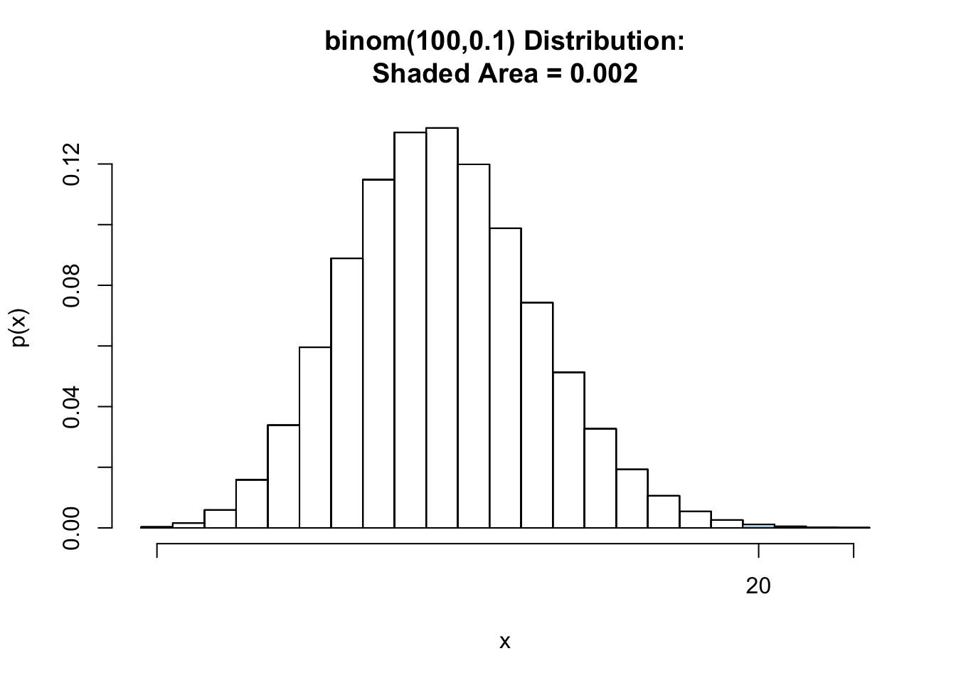
[1] 0.001978561
With the resulting small risk of a wrong conclusion, it would seem safe to reject the hypothesis that p = 0.10.
由于得出错误结论的风险很小,因此可以安全地拒绝 p = 0.10 的假设。
In other words, rejection of a hypothesis tends to all but rule out the hypothesis. On the other hand, it is very important to emphasize that acceptance or, rather, failure to reject does not rule out other possibilities.
换句话说,拒绝一个假设,就等于排除了这个假设。另一方面,非常重要的是要强调,接受或者更确切地说,不拒绝并不排除其他可能性。
The foregoing implies that when the data analyst formalizes experimental evidence on the basis of hypothesis testing, the formal statement of the hypothesis is very important.
上述情况表明,当数据分析者在假设检验的基础上将实验证据形式化时,对假设的形式化陈述是非常重要的。
# Elements of a hypothesis test 假设检验的要素
# Hypotheses 假设
null hypothesis, denoted by
零假设,表示为
alternative hypothesis, denoted by
替代假设,表示为
In our binomial example, we may state
在二项式的例子中,我们可以说
Now 12 defective items out of 100 does not refute , so the conclusion is “fail to reject ”. However, if the data produce 20 out of 100 defective items, then the conclusion is “reject ” in favor of .
现在 100 件中有 12 件有缺陷并不能反驳,所以结论是 “不能拒绝”。然而,如果 100 个数据中产生 20 个缺陷项,那么结论是 “拒绝” 而支持。
# Test Statistic and Critical Region 检验统计量和临界区
# Discrete Case Study 离散案例研究
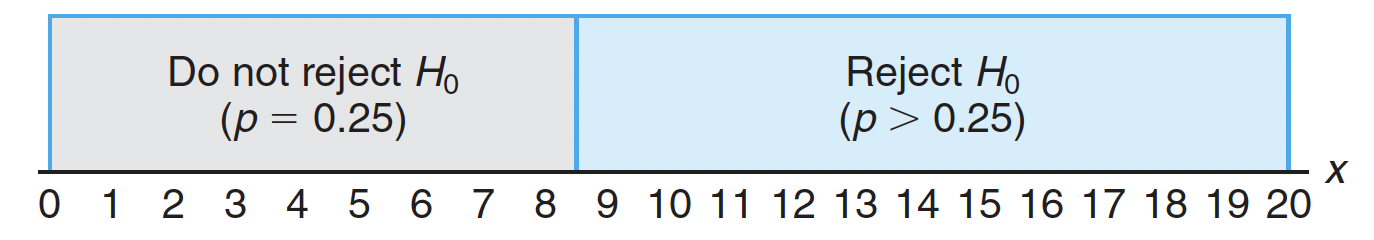
A certain type of cold vaccine is known to be only 25% effective after a period of 2 years.
已知某种类型的感冒疫苗在 2 年后只有 25% 的有效性。
To determine if a new and somewhat more expensive vaccine is superior in providing protection against the same virus for a longer period of time, suppose that 20 people are chosen at random and inoculated.
为了确定一种新的、价格稍高的疫苗是否在更长时间内针对同一病毒提供更好的保护,假设随机选择 20 人进行接种。
If more than 8 of those receiving the new vaccine surpass the 2-year period without contracting the virus, the new vaccine will be considered superior to the one presently in use.
如果接受新疫苗的人中有超过 8 人超过 2 年没有感染病毒,则新疫苗将被视为优于目前使用的疫苗。
We are essentially testing the null hypothesis that the new vaccine is equally effective after a period of 2 years as the one now commonly used.
我们基本上是在检验零假设,即新疫苗在 2 年后与现在常用的疫苗同样有效。
The alternative hypothesis is that the new vaccine is in fact superior.
另一种假设是,新疫苗实际上更优越。
The test statistic on which we base our decision is , the number of individuals in our test group who receive protection from the new vaccine for a period of at least 2 years.
我们做出决定所依据的检验统计量是,即测试组中获得至少 2 年新疫苗保护的人数。
The possible values of , from 0 to 20, are divided into two groups: those numbers less than or equal to 8 and those greater than 8. All possible scores greater than 8 constitute the critical region.
可能的值,从 0 到 20,分为两组:小于等于 8 和大于 8 的数值。所有可能的大于 8 的数值构成临界区。
The last number that we observe in passing into the critical region is called the critical value.
最后一个进入临界区的数值称为临界值。
In our illustration, the critical value is the number 8.
在我们的图例中,临界值是 8。
Therefore, if , we reject in favor of the alternative hypothesis .
因此,如果,我们拒绝 而支持另一种假设。
If , we fail to reject .
如果,我们则无法拒绝。
# Continuous Case Study 连续案例研究
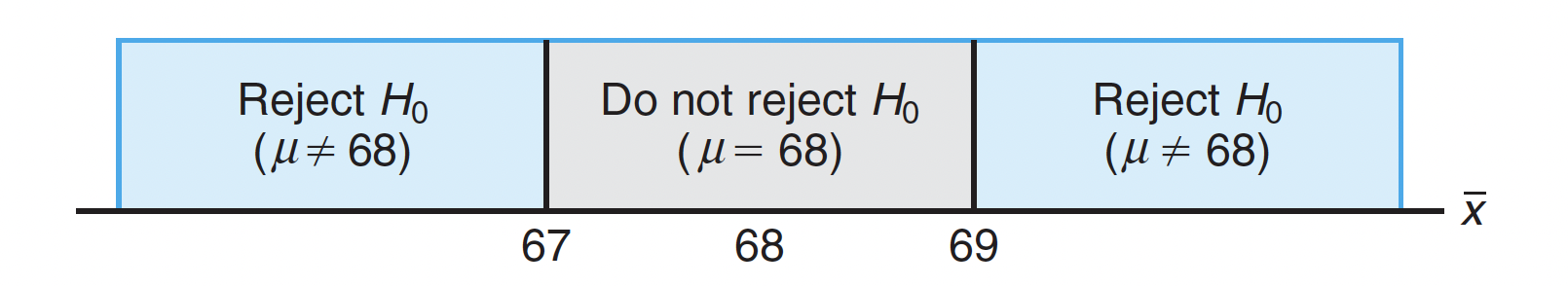
Consider the null hypothesis that the average weight of male students in a certain college is 68 kilograms against the alternative hypothesis that it is unequal to 68.
考虑某大学男学生平均体重为 68 公斤的零假设与不等于 68 的备择假设。
That is, we wish to test
即,我们希望检验
The alternative hypothesis allows for the possibility that or .
备择假设允许以下可能性 或者 。
Sample mean that falls close to the hypothesized value of 68 would be considered evidence in favor of .
样本均值接近假设值 68 将被视为支持 的证据。
On the other hand, a sample mean that is considerably less than or more than 68 would be evidence inconsistent with and therefore favoring .
另一方面,样本均值远小于或大于 68,将是与 不一致的证据,因此有利于。
The sample mean is the test statistic in this case.
在本例中,样本均值是检验统计量。
A critical region for the test statistic might arbitrarily be chosen to be the two intervals and .
检验统计量的临界区可以任意选择为两个区间 和 。
The non-rejection region will then be the interval .
非拒绝区将是区间 。
# One- and Two-Tailed Tests 单尾和双尾检验
A test of any statistical hypothesis where the alternative is one sided, such as
对任何统计假设的检验,其中备选方案是单边的,如
or perhaps
is called a one-tailed test.
称为单尾检验。
Generally, the critical region for the alternative hypothesis lies in the right tail of the distribution of the test statistic, while the critical region for the alternative hypothesis lies entirely in the left tail.
一般来说,替代假设的临界区 位于检验统计量分布的右尾,而替代假设的临界区 完全位于左尾。
(In a sense, the inequality symbol points in the direction of the critical region.)
从某种意义上说,不等式符号指向临界区的方向。
A test of any statistical hypothesis where the alternative is two sided, such as
对任何统计假设的检验,其中备选方案是两侧的,例如
is called a two-tailed test.
称为双尾检验。
Question: In the above two case studies, which one is a one-tailed test? Which one is a two-tailed test?
在以上两个案例研究中,哪一个是单尾测试?哪一个是双尾测试?
# In-Class Exercise: Determine the hypotheses, test statistics, critical region
A manufacturer of a certain brand of rice cereal claims that the average saturated fat content does not exceed 1.5 grams per serving. State the null and alternative hypotheses to be used in testing this claim and determine where the critical region
is located.
某品牌米糊制造商声称每份平均饱和脂肪含量不超过 1.5 克。陈述用于测试此声明的无效假设和替代假设,并确定关键区域位于何处。A real estate agent claims that 60% of all private residences being built today are 3-bedroom homes. To test this claim, a large sample of new residences is inspected; the proportion of these homes with 3 bedrooms is recorded and used as the test statistic. State the null and alternative hypotheses to be used in this test and determine the location of the critical region.
一位房地产经纪人声称,当今建造的所有私人住宅中有 60% 是三居室住宅。为了检验这一说法,我们检查了大量新住宅样本;记录这些拥有 3 间卧室的房屋的比例并用作测试统计数据。陈述要在此测试中使用的原假设和替代假设,并确定关键区域的位置。
# Hypothesis Testing 假设检验
# Approach to Hypothesis Testing with Fixed Probability 固定概率 的假设检验方法
State the null and alternative hypotheses.
陈述零假设和替代假设。Choose a fixed significance level .
选择一个固定的显著性水平。Choose an appropriate test statistic and establish the critical region based on .
选择适当的检验统计量并基于 建立临界区。Reject if the computed test statistic is in the critical region. Otherwise, do not reject.
如果计算的测试统计量在临界区,则拒绝。否则,不要拒绝。Draw scientific or engineering conclusions.
得出科学或工程结论。
# Tests on a Single Mean (Variance Known) 单一均值检验(方差已知)
The model for the underlying situation centers around an experiment with representing a random sample from a distribution with mean and variance .
潜在情况的模型围绕一个实验,用 代表一个来自均值为 和方差 的分布的随机样本。
Consider first the hypothesis
首先考虑假设
The appropriate test statistic should be based on the random variable .
适当的检验统计量应基于随机变量。
This is a two-tailed test, given , we should reject , if
这是一个双尾检验,给定 ,如果
我们应该拒绝 。
# Example 1
A manufacturer of sports equipment has developed a new synthetic fishing line that the company claims has a mean breaking strength of 8 kilograms with a standard deviation of 0.5 kilogram.
一家运动器材制造商开发了一种新的合成鱼线,该公司称其平均断裂强度为 8 公斤,标准差为 0.5 公斤。
Test the hypothesis that kilograms against the alternative that kilograms if a random sample of 50 lines is tested and found to have a mean breaking strength of 7.8 kilograms.
如果随机抽取 50 条线进行测试,发现其平均断裂强度为 7.8 公斤,则测试假设kg 与备选假设kg。
Use a 0.01 level of significance.
使用 0.01 的显著性水平。
We get critical region first.
首先得到临界区。
alpha <- 0.01 | |
qnorm(alpha/2) # -z_{alpha/2} |
[1] -2.575829
Critical region: and
临界区: 和
xbar <- 7.8 | |
mu_0 <- 8 | |
sigma <- 0.5 | |
n <- 50 | |
z <- (xbar - mu_0)/(sigma/sqrt(n)) | |
z |
[1] -2.828427
, we should reject .
To get critical region in Python , We need scipy package.Python 中想要获得临界区,需要 scipy 包。
We can get the same region using norm.ppf .
可以使用 norm.ppf 。
from scipy.stats import norm | |
norm.ppf(0.01/2) |
-2.575829303548901
Question: What about one-tailed test?
# Example 2
A random sample of 100 recorded deaths in the United States during the past year showed an average life span of 71.8 years.
过去一年在美国记录的 100 例死亡的随机样本显示平均寿命为 71.8 岁。
Assuming a population standard deviation of 8.9 years, does this seem to indicate that the mean life span today is greater than 70 years?
假设人口标准差为 8.9 岁,这是否表明今天的平均寿命大于 70 岁?
Use a 0.05 level of significance.
使用 0.05 的显著性水平。
xbar <- 71.8 | |
mu_0 <- 70 | |
sigma <- 8.9 | |
n <- 100 | |
z <- (xbar - mu_0)/(sigma/sqrt(n)) | |
z |
[1] 2.022472
alpha <- 0.05 | |
qnorm(1-alpha) # z_{alpha} |
[1] 1.644854
Therefore, we reject and conclude that the mean life span today is greater than 70 years.
因此,我们拒绝 并得出结论,今天的平均寿命大于 70 岁。
# Use of P-Values
- Definition
- A P-value is the lowest level (of significance) at which the observed value of the test statistic is significant.
P 值是检验统计量的观察值达到显著意义的最低水平(显著性)。
# Revisit Example 1
A manufacturer of sports equipment has developed a new synthetic fishing line that the company claims has a mean breaking strength of 8 kilograms with a standard deviation of 0.5 kilogram.
一家运动器材制造商开发了一种新的合成钓鱼线,该公司声称其平均断裂强度为 8 公斤,标准偏差为 0.5 公斤。
Test the hypothesis that kilograms against the alternative that kilograms if a random sample of 50 lines is tested and found to have a mean breaking strength of 7.8 kilograms.
如果随机抽取 50 条线进行测试,发现其平均断裂强度为 7.8 公斤,则测试假设kg 与备选假设kg。
We can still construct the same hypotheses.
仍然可以构造相同的假设。
Since the test in this example is two tailed, the desired -value is twice the area of the shaded region to the left of .
由于本示例中的测试是两尾的,因此所需的 值是 左侧阴影区域面积的两倍。
We have
pnormGC(c(-2.83,2.83),region = "outside",graph = TRUE) |
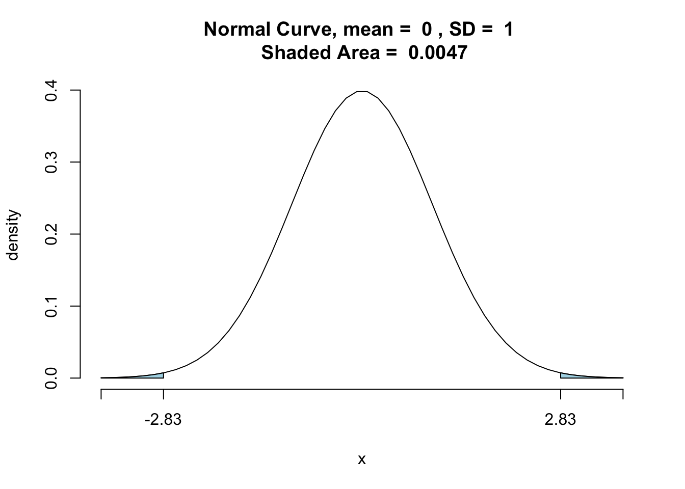
[1] 0.0046548
Based on the very small p-value, we should reject .
基于非常小的 p 值,应该拒绝 .
We can also check p value in python .
from scipy.stats import norm | |
1-(norm.cdf(2.83)-norm.cdf(-2.83)) |
0.0046548004134630006
We can also get the small p-value, we should rejcet .
# Revisit Example 2
A random sample of 100 recorded deaths in the United States during the past year showed an average life span of 71.8 years.
Assuming a population standard deviation of 8.9 years, does this seem to indicate that the mean life span today is greater than 70 years?
Use a 0.05 level of significance.
We can still construct the same hypotheses.
仍然可以构造相同的假设。
The p-value corresponding to is given by the area of the shaded region in the following figure.
对应的 p 值由下图中阴影区域的面积给出。
We have
As a result, the evidence in favor of is even stronger than that suggested by a 0.05 level of significance.
支持 的证据甚至比 0.05 显著性水平所建议的还要强。
pnormGC(2.02,region = "above",graph = TRUE) |
[1] 0.02169169
We can also use Python to get p value.
1 - norm.cdf(2.02) |
0.02169169376764679
P value is less than 0.05.
We should reject .
# In-class Exercise
In a research report, Richard H. Weindruch of the UCLA Medical School claims that mice with an average life span of 32 months will live to be about 40 months old when 40% of the calories in their diet are replaced by vitamins and protein.
平均寿命为 32 个月的老鼠,当它们饮食中 40% 的卡路里被维生素和蛋白质所取代时,它们可以活到 40 个月大。
Is there any reason to believe that if 64 mice that are placed on this diet have an average life of 38 months with a standard deviation of 5.8 months? Use a P-value in your conclusion.
如果 64 只老鼠接受这种饮食,平均寿命为 38 个月,标准差为 5.8 个月,那么有没有理由相信 ?在结论中用 p 值。An electrical firm manufactures light bulbs that have a lifetime that is approximately normally distributed with a mean of 800 hours and a standard deviation of 40 hours.
一家电气公司生产的灯泡寿命大约为正态分布,平均 800 小时,标准差为 40 小时。
Test the hypothesis that μ = 800 hours against the alternative, hours, if a random sample of 30 bulbs has an average life of 788 hours.
如果随机抽取 30 个灯泡,平均寿命为 788 小时,则检验 小时的假设,
Use a P-value in your answer
xbar <- 788 | |
n <- 30 | |
mu0 <- 800 | |
sigma <- 40 | |
zstats <- (xbar-mu0)/(sigma/sqrt(n)) | |
zstats |
[1] -1.643168
pnormGC(c(zstats,-zstats),region = "outside",graph = TRUE) |
[1] 0.1003482
Not reject
xbar <- 38 | |
n <- 64 | |
mu0 <- 40 | |
sigma <- 5.8 | |
zstats <- (xbar-mu0)/(sigma/sqrt(n)) | |
zstats |
[1] -2.758621
pnormGC(zstats,region = "below",graph = TRUE) |
[1] 0.002902293
Reject
# Tests on a Single Mean (Variance Unknown) 单一均值检验(方差未知)
For the two-sided hypothesis
对于双边假设
We reject at significance level , When
the computed -statistic
exceeds or is less than .
当计算统计量 超过 或少于 ,在显著性水平 拒绝。
# Example 3
Data are collected on a neutral substance (pH = 7.0).
收集关于中性物质(pH = 7.0)的数据。
A sample of the measurements were taken with the data as follows:
使用以下数据进行测量的样本:
It is, then, of interest to test
phmeter <-c(7.07,7.00,7.10,6.97,7.00,7.03,7.01,7.01, 6.98,7.08) | |
xbar <- mean(phmeter) | |
s <- sd(phmeter) | |
n <- length(phmeter) | |
tvalue <- (xbar -7)/(s/sqrt(n)) | |
tvalue |
[1] 1.79541
#get P-Value | |
ptGC(c(-tvalue,tvalue),region = "outside",df = n-1,graph = TRUE) |
[1] 0.106159
We can also use t.test here.
#Need to specify mu | |
t.test(phmeter, mu = 7) |
    One Sample t-test

data:  phmeter
t = 1.7954, df = 9, p-value = 0.1062
alternative hypothesis: true mean is not equal to 7
95 percent confidence interval:
 6.993501 7.056499
sample estimates:
mean of x
    7.025
from scipy import stats | |
import numpy as np | |
phmeter = np.array([7.07,7.00,7.10,6.97,7.00,7.03,7.01,7.01, 6.98,7.08]) | |
stats.ttest_1samp(phmeter, 7.0) |
Ttest_1sampResult(statistic=1.7954096195592317, pvalue=0.10615895425089732)
Should we reject or not reject ?
If we consider , we should not reject .
Notice that the sample size of 10 is rather small.
请注意,10 的样本量相当小。
An increase in sample size (perhaps another experiment) may sort things out.
增加样本量(也许是另一个实验)可能会解决问题。
Note: How to choose a good sample size is an advanced topic.
如何选择一个好的样本量是一个高级话题。
# In-Class Exercise
Test the hypothesis that the average content of containers of a particular lubricant is 10 liters if the contents of a random sample of 10 containers are 10.2, 9.7, 10.1, 10.3, 10.1, 9.8, 9.9, 10.4, 10.3, and 9.8 liters.
如果 10 个容器的随机样本的含量为...,则测试特定润滑剂容器的平均含量为 10 升的假设。
Use a 0.01 level of significance and assume that the distribution of contents is normal.
使用 0.01 显著性水平,并假设为正态分布。
lubricant <-c(10.2, 9.7, 10.1, 10.3, 10.1, 9.8, 9.9, 10.4, 10.3, 9.8 ) | |
t.test(lubricant, mu = 10,conf.level = 0.99) |
    One Sample t-test

data:  lubricant
t = 0.77174, df = 9, p-value = 0.46
alternative hypothesis: true mean is not equal to 10
99 percent confidence interval:
  9.807338 10.312662
sample estimates:
mean of x
    10.06
Based on the evidence, we can not reject .
# Tests on Two Means (Variances Known) 两种均值的检验(方差已知)
For the two-sided hypothesis
对于双边假设
We reject at significance level , When
the computed -statistic
exceeds or is less than .
当计算统计量 超过 或少于 ,在显著性水平 拒绝。
# Example 4
A study was conducted in which two types of engines, and were compared.
进行了一项研究,对两种类型的发动机, 和,进行了比较。
Gas mileage, in miles per gallon, was measured.
汽油里程以每加仑英里为单位进行了测量。
Fifty experiments were conducted using engine type and 75 experiments were done with engine type .
使用 发动机进行了 50 次试验,使用 发动机进行了 75 次试验。
The gasoline used and other conditions were held constant.
使用的汽油和其他条件保持不变。
The average gas mileage was 36 miles per gallon for engine and 42 miles per gallon for engine .
发动机 的平均燃油里程为 36 英里 / 加仑,发动机 的平均燃油里程为 42 英里 / 加仑。
Assume that the population standard deviations are 6 and 8 for engines and respectively.
假设发动机 的总体标准差为 6 英里 / 加仑,发动机 的总体标准差为 8 英里 / 加仑。
Let . Can we say these two engines have the same gas mileage?
设\α=0.05。可以说这两台发动机的油耗是一样的吗?
xAbar <- 36 | |
xBbar <- 42 | |
sigmaA <-6 | |
sigmaB <- 8 | |
nA <- 50 | |
nB <- 75 | |
alpha <- 0.05 | |
zvalue <- (xAbar-xBbar)/sqrt(sigmaA^2/nA +sigmaB^2/nB) | |
zvalue |
[1] -4.783446
zalphaOver2 <- qnorm(1-alpha/2) | |
zalphaOver2 |
[1] 1.959964
As the value is less than , we should reject .
由于该值小于 ,应该拒绝 。
# Tests on Two Means (Unknown But Equal Variance) 两个均值的检验(方差未知但相等)
For the two-sided hypothesis
对于双边假设
We reject at significance level , When
the computed -statistic
where
exceeds or is less than .
当计算统计量 超过 或少于 ,在显著性水平 拒绝。
# Example 5
In a study conducted at Virginia Tech on the development of ectomycorrhizal, a symbiotic relationship between the roots of trees and a fungus, in which minerals are transferred from the fungus to the trees and sugars from the trees to the fungus, 20 northern red oak seedlings exposed to the fungus Pisolithus tinctorus were grown in a greenhouse.
关于外生菌根发展的研究中,研究树根和真菌之间的共生关系,其中矿物质从真菌转移到树木,糖从树转移到真菌,20 棵暴露在真菌中的幼苗生长在温室中。
All seedlings were planted in the same type of soil and received the same amount of sunshine and water.
所有幼苗都种植在同一类型的土壤中,并得到同样数量的阳光和水。
Half received no nitrogen at planting time, to serve as a control, and the other half received 368 ppm of nitrogen in the form NaNO_3_.
一半在种植时没有接受氮作为对照组,另一半从 NANO_3_接受 368ppm 的氮。
The stem weights, in grams, at the end of 140 days were recorded as follows:
在 140 天结束时,以克为单位的茎重量记录如下:
No Nitrogen:
0.32 0.53 0.28 0.37 0.47 0.43 0.36 0.42 0.38 0.43

Nitrogen:
0.26 0.43 0.47 0.49 0.52 0.75 0.79 0.86 0.62 0.46
Hypothesis Test:
假设检验:
where the population means indicate mean weights.
其中总体均值表示平均权重。
Assume the populations to be normally distributed with equal variances.
假设总体呈正态分布,方差相等。
noNitro<- c(0.32,0.53 ,0.28, 0.37, 0.47, 0.43, 0.36, 0.42,0.38,0.43) | |
x1 <- mean(noNitro) | |
s1 <- sd(noNitro) | |
n1 <- 10 | |
Nitro<- c(0.26,0.43,0.47,0.49,0.52,0.75,0.79,0.86, 0.62,0.46) | |
x2 <- mean(Nitro) | |
s2<- sd(Nitro) | |
n2<- 10 | |
sp<- sqrt(((n1-1)*s1^2 + (n2-1)*s2^2)/(n1+n2-2)) | |
tvalue <- (x1-x2)/(sp*sqrt(1/n1+1/n2)) | |
tvalue |
[1] -2.619094
alpha <- 0.05 | |
qt(alpha/2,n1+n2-2) |
[1] -2.100922
As tvalue , we reject .
Yes!
We can use two sample t-test.
可以使用双样本检验。
Don't forget to add the condition var.equal = TURE .
t.test(noNitro,Nitro, var.equal = TRUE, conf.level = .95) |
    Two Sample t-test

data:  noNitro and Nitro
t = -2.6191, df = 18, p-value = 0.01739
alternative hypothesis: true difference in means is not equal to 0
95 percent confidence interval:
 -0.29915788 -0.03284212
sample estimates:
mean of x mean of y
    0.399     0.565
ptGC(c(tvalue,-tvalue),region = "outside",df = n1+n2-2,graph = TRUE) |
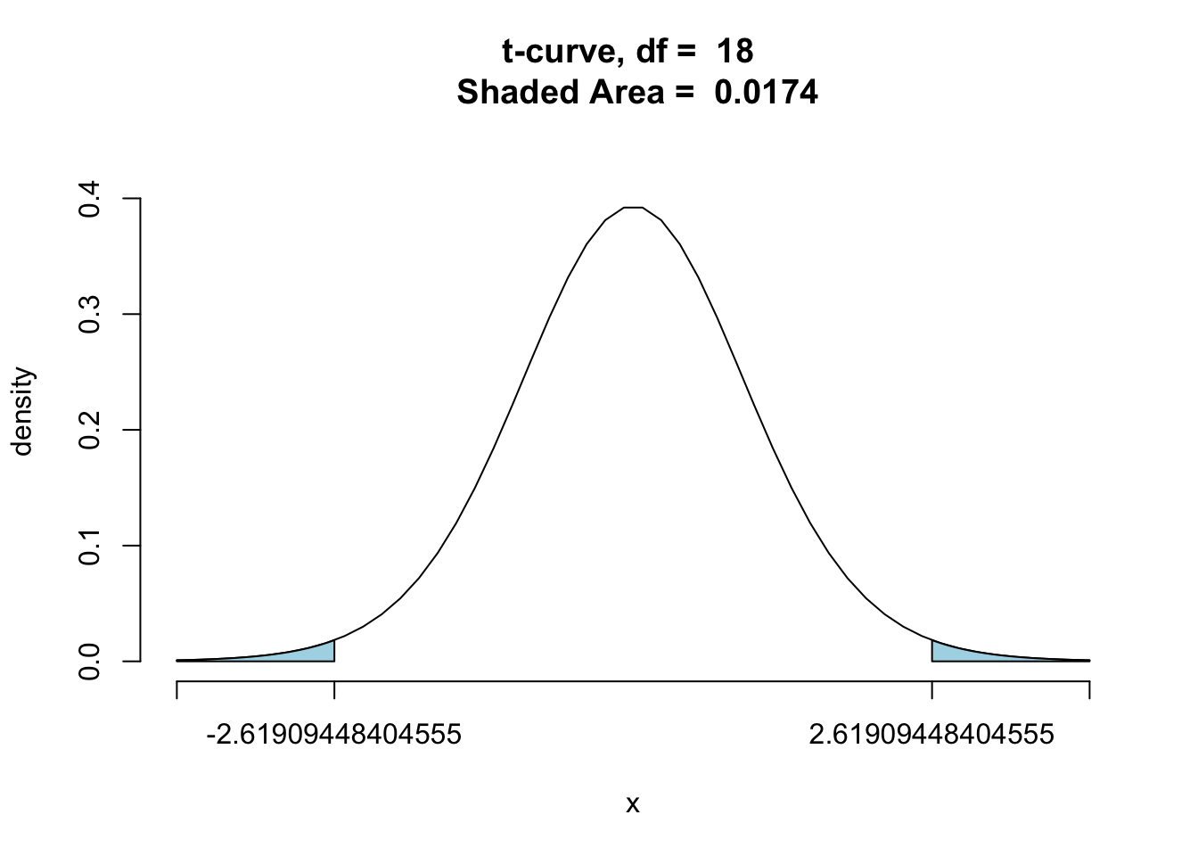
[1] 0.01738648
Here we make an assumption that the variances are equal. Does that make sense?
这里假设方差相等。那有意义吗?
boxplot(noNitro,Nitro) |
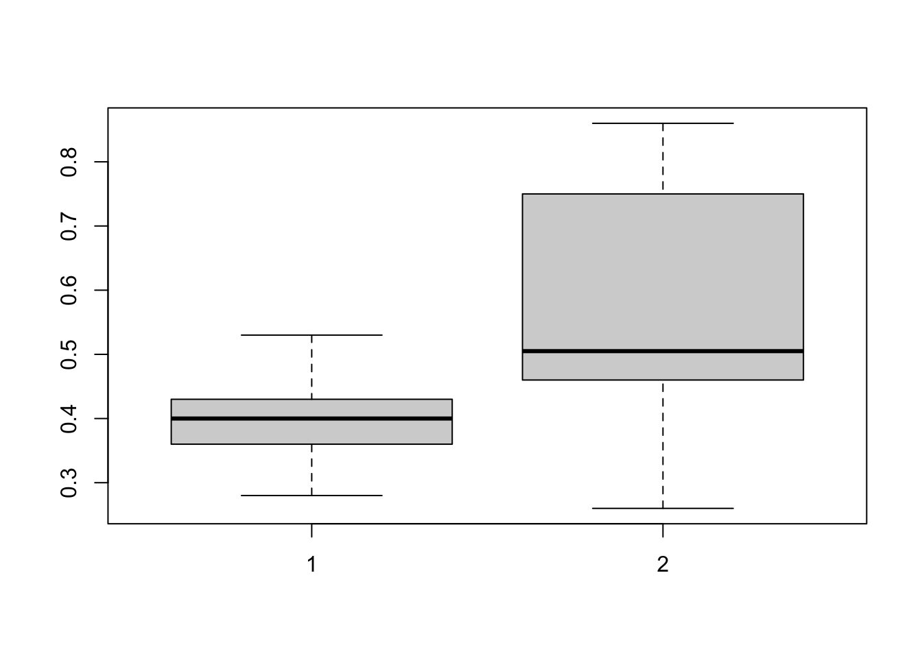
Can we do a mean test with different variances? Yes!
可以做一个不同方差的均值检验吗?是的!
t.test(noNitro,Nitro, var.equal = FALSE, conf.level = .95) |
    Welch Two Sample t-test

data:  noNitro and Nitro
t = -2.6191, df = 11.673, p-value = 0.02286
alternative hypothesis: true difference in means is not equal to 0
95 percent confidence interval:
 -0.30452438 -0.02747562
sample estimates:
mean of x mean of y
    0.399     0.565
No matter which method we choose, we should reject .
无论选择哪种方式,都应该拒绝。
How to do a two samples test in Python ?
如何用 Python 进行双样本检验?
Let's try the same variances first.
先尝试等方差
noNitro = np.array([0.32,0.53 ,0.28, 0.37, 0.47, 0.43, 0.36, 0.42,0.38,0.43]) | |
nitro = np.array([0.26,0.43,0.47,0.49,0.52,0.75,0.79,0.86, 0.62,0.46]) | |
stats.ttest_ind(noNitro, nitro, equal_var=True) |
Ttest_indResult(statistic=-2.6190944840455472, pvalue=0.017386483684799125)
We can also assume the variances are not equal.
也可以假设方差不相等。
stats.ttest_ind(noNitro, nitro, equal_var=False) |
Ttest_indResult(statistic=-2.6190944840455472, pvalue=0.022863946155002354)
Therefore, we also should reject .
因此,我们也应该拒绝 。
# In-class Exercise: Tests on Two Means (Unknown But Not Equal Variance)
A study was conducted by the Department of Zoology at Virginia Tech to determine if there is a significant difference in the density of organisms at two different stations located on Cedar Run, a secondary stream in the Roanoke River drainage basin.
一项研究,以确定位于河流上的两个不同站点的生物密度是否存在显着差异。
Sewage from a sewage treatment plant and overflow
from the Federal Mogul Corporation settling pond enter the stream near its headwaters.
来自污水处理厂的污水和来自沉淀池的溢流进入其源头附近的河流。
The following data give the density measurements, in number of organisms per square meter, at the two collecting stations:
以下数据给出了两个收集站每平方米生物体数量的密度测量值:
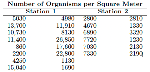
Can we conclude, at the 0.05 level of significance, that the average densities at the two stations are equal?
我们能否在 0.05 的显著性水平上得出两个站点的平均密度相等的结论?
Assume that the observations come from normal populations with different variances.
假设观测值来自具有不同方差的正态总体。
stat1 <-c(5030,4980,13700,11910,10730,8130,11400,26850,860,17660,2200,22800,4250,1130,15040,1690) | |
stat2 <-c(2800,2810,4670,1330,6890,3320,7720,1230,7030,2130,7330,2190) | |
t.test(stat1,stat2,conf.level = 0.95, var.equal = FALSE) |
    Welch Two Sample t-test

data:  stat1 and stat2
t = 2.7578, df = 18.781, p-value = 0.01261
alternative hypothesis: true difference in means is not equal to 0
95 percent confidence interval:
  1389.003 10164.331
sample estimates:
mean of x mean of y
 9897.500  4120.833
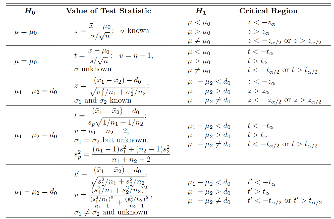
# A Table of Hypothesis Tests on Means 均值假设检验表
# Test on a Single Proportion 单一比例检验
For the two-sided hypothesis
对于双边假设
The appropriate random variable on which we base our decision criterion is the binomial random variable , although we could just as well use the statistic .
基于决策标准的适当随机变量是二项式随机变量 ,虽然也可以使用统计量 。
Values of that are far from the mean will lead to the rejection of the null hypothesis.
的值远离平均值 将导致拒绝零假设。
Because is a discrete binomial variable, it is unlikely that a critical region can be established whose size is exactly equal to a pre-specified value of .
因为 是一个离散的二项式变量,不可能建立一个临界区,其大小完全等于预先指定的值 。
For this reason it is preferable, in dealing with small samples, to base our decisions on P-values.
出于这个原因,在处理小样本时,决策最好基于 P 值。
At the -level of significance, we compute
在 - 显著性水平,计算
or
and reject in favor of if the computed P-value is less than or equal to .
如果计算出的 P 值小于或等于 ,拒绝 有利于 。
# Example 6
In a random sample of families owning television sets in the city of Hamilton, Canada, it is found that subscribe to HBO.
在 加拿大汉密尔顿市拥有电视机的家庭随机样本中发现, 订阅了 HBO 的家庭是 。
Suppose we make the conjecture, the proportion of families with television sets in this city that subscribe to HBO is 0.7.
假设一个猜想,这个城市有电视机的家庭订阅 HBO 的比例是 0.7。
We have the following hypotheses.
我们有以下假设。
# alpha is still 0.05 | |
prop.test(x = 340, n = 500, p = 0.7, alternative = "two.sided", conf.level = 0.95) |
    1-sample proportions test with continuity correction

data:  340 out of 500
X-squared = 0.85952, df = 1, p-value = 0.3539
alternative hypothesis: true p is not equal to 0.7
95 percent confidence interval:
 0.6368473 0.7203411
sample estimates:
   p
0.68
How to get p-value?
2*pbinomGC(340,region = "below", size = 500, prob = 0.7,graph = TRUE) |
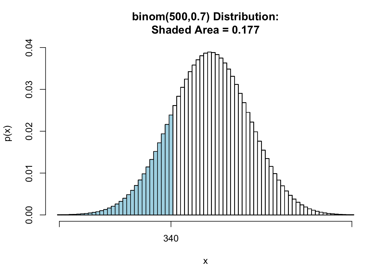
[1] 0.3533839
We can find p-value is much larger than , we should not reject .
可以发现 p 值远大于 ,我们不应该拒绝.
What about
prop.test(x = 340, n = 500, p = 0.7, alternative = "greater", conf.level = 0.95) |
    1-sample proportions test with continuity correction

data:  340 out of 500
X-squared = 0.85952, df = 1, p-value = 0.8231
alternative hypothesis: true p is greater than 0.7
95 percent confidence interval:
 0.6437733 1.0000000
sample estimates:
   p
0.68
As this one-tailed test,so the p value is
由于这是个单尾检验,所以 p 值是
pbinomGC(340,region = "above", size = 500, prob = 0.7,graph = TRUE) |
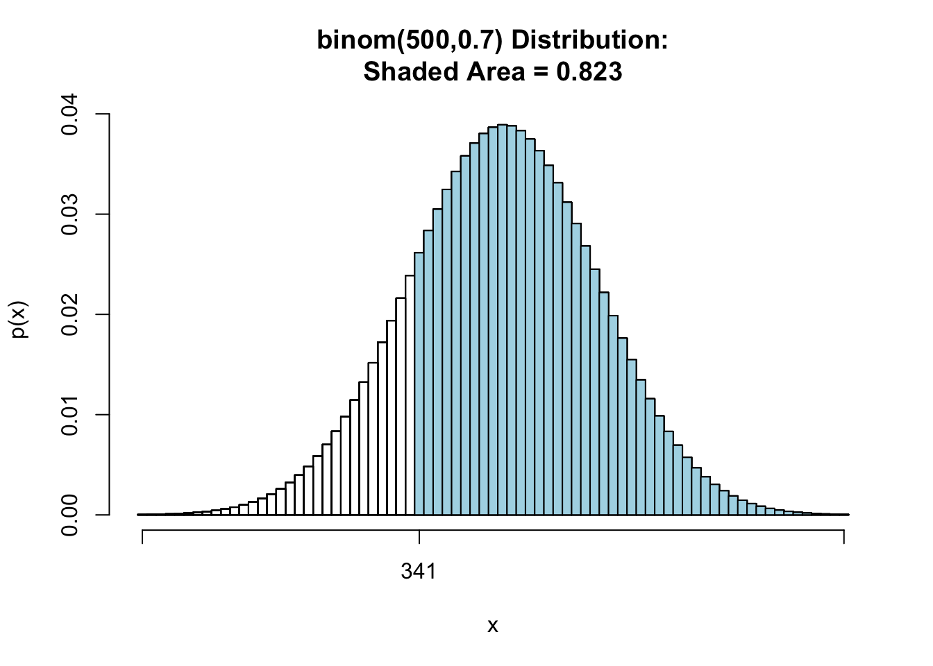
[1] 0.8233081
We also can find p-value is much larger than , we should not reject .
发现 p 值远大于 ,我们不应该拒绝 。
# In-class Exercise: Test on a Single Proportion.
A commonly prescribed drug for relieving nervous tension is believed to be only 60% effective.
一种用于缓解神经紧张的常用处方药据信只有 60% 有效率。
Experimental results with a new drug administered to a random sample of 100 adults who were suffering from nervous tension show that 70 received relief.
对 100 名患有神经紧张的成年人随机服用一种新药的实验结果表明,其中 70 人得到了缓解。
Is this sufficient evidence to conclude that the new drug is superior to the one commonly prescribed? (NO/YES: Use a 0.05 level of significance.)
这是否足以得出结论,新药优于常用处方药?(否 / 是:使用 0.05 的显着性水平。)
When is large, we can use the normal approximation.
很大时,我们可以使用正态近似。
The z-value for testing is given by
用于测试 的 z 值为
, which is a value of the standard normal variable .
这是标准正态变量的一个值
Hence, for a two-tailed test at the -level of significance, the critical region is or .
因此,对于 显著性水平的双尾检验,临界区是 or 。
For the one-sided alternative , the critical region is , and for the alternative , the critical region is .
对于单边备择项 ,临界区是 ,而对于备择项 ,临界区是 。
xhat <- 70 | |
n <- 100 | |
phat <- xhat/n | |
p0 <- 0.6 | |
zvalue <- (phat-p0)/(sqrt(p0*(1-p0)/n)) | |
zvalue |
[1] 2.041241
alpha <- 0.05 | |
zalpha <- qnorm(1-alpha) | |
zalpha |
[1] 1.644854
#p value | |
1-pnorm(zvalue) |
[1] 0.02061342
It is easily to see , we should reject .
p value is 0.0206.
prop.test(x = 70, n = 100, p = 0.6, alternative = "greater", conf.level = 0.95) |
    1-sample proportions test with continuity correction

data:  70 out of 100
X-squared = 3.7604, df = 1, p-value = 0.02624
alternative hypothesis: true p is greater than 0.6
95 percent confidence interval:
 0.6149607 1.0000000
sample estimates:
  p
0.7
We should reject .
# Two Samples: Tests on Two Proportions 两个样本:两个比例的检验
In general, we wish to test the null hypothesis that two proportions, or binomial parameters, are equal.
一般来说,我们希望检验两个比例或二项式参数相等的零假设。
That is, we are testing against one of the alternatives , , or .
也就是说,针对备选方案 , , 或 之一,检验 。
The z-value for testing is determined from the formula
用于测试 的 z 值
由公式确定,其中
,where .
The critical regions for the appropriate alternative hypotheses are set up as before, using critical points of the standard normal curve.
如前所述,使用标准正态曲线的临界点设置适当替代假设的临界区域。
Hence, for the alternative at the -level of significance, the critical region is or .
因此,备择假设 在 显著性水平的临界区为 或 。
For a test where the alternative is , the critical region is , and when the alternative is , the critical region is .
对于 ,临界区域为 ;对于 ,临界区域为 。
# Example 7
A vote is to be taken among the residents of a town and the surrounding county to determine whether a proposed chemical plant should be constructed.
在一个城镇和周围县的居民中进行投票,以决定是否应该建造一个拟议的化工厂。
The construction site is within the town limits, and for this reason many voters in the county believe that the proposal will pass because of the large proportion of town voters who favor the construction.
建筑工地在城镇范围内,因此许多县里的选民相信,由于大部分城镇选民支持建筑工程,这项提案将获得通过。
To determine if there is a significant difference in the proportions of town voters and county voters favoring the proposal, a poll is taken.
为了确定支持该提案的城镇选民和县选民的比例是否存在显著差异,进行了一次民意调查。
If 120 of 200 town voters favor the proposal and 240 of 500 county residents favor it, would you agree that the proportion of town voters favoring the proposal is higher than the proportion of county voters?
如果 200 个乡镇选民中有 120 个支持该提案,500 个乡镇居民中有 240 个支持该提案,你是否同意乡镇选民支持该提案的比例高于乡镇选民的比例?
Use an level of significance.
x1 <- 120 | |
n1 <- 200 | |
x2 <- 240 | |
n2 <- 500 | |
p1hat <- x1/n1 | |
p2hat <- x2/n2 | |
phat <- (x1+x2)/(n1+n2) | |
#get z statistic | |
zvalue <- (p1hat-p2hat)/(sqrt(phat*(1-phat)*(1/n1+1/n2))) | |
zvalue |
[1] 2.86972
#get critical region | |
alpha <- 0.05 | |
zalpha <- qnorm(1-alpha) | |
zalpha |
[1] 1.644854
#get p-value | |
1-pnorm(zvalue) |
[1] 0.002054176
Therefore, we reject and agree that the proportion of town voters favoring the proposal is higher than the proportion of county voters.
因此,我们拒绝 ,并同意城镇选民赞成该提案的比例高于县选民的比例。
Can we use prop.test ? Yes
# alpha is still 0.05 | |
prop.test(x = c(120,240), n = c(200,500), alternative = "greater", conf.level = 0.95) |
    2-sample test for equality of proportions with continuity correction

data:  c out of c120 out of 200240 out of 500
X-squared = 7.7619, df = 1, p-value = 0.002668
alternative hypothesis: greater
95 percent confidence interval:
 0.04869691 1.00000000
sample estimates:
prop 1 prop 2
  0.60   0.48
We also can find p-value is much smaller than , we should reject .
我们还可以发现 p 值远小于 ,我们应该拒绝 。
# Two-Sample Tests Concerning Variances 关于方差的两样本检验
In this section, we are concerned with testing hypotheses concerning comparison of population variances or standard deviations.
在本节中,我们将检验有关总体方差或标准差比较的假设。
Attention is focused on comparative experiments between methods or processes, where inherent reproducibility or variability must formally be compared.
注意力集中在方法或过程之间的比较实验上,固有的重现性或变异性必须进行形式上的比较。
In addition, to determine if the equal variance assumption is violated, a test comparing two variances is often applied prior to conducting a t-test on two means.
此外,为了确定是否违反了等方差假设,在对两个平均值进行 t 检验之前,通常会进行一个比较两个方差的检验。
We shall test the null hypothesis that against one of the usual alternatives
假设零假设 为 ,通常的备择假设之一为
For independent random samples of sizes and , respectively, from the two populations, the f-value for testing is the ratio
对于大小为 和 的分别来自两个群体的独立随机样本,用于检验 的 f 值是比率
, where and are the variances computed from the two samples.
和 是从两个样本计算的方差。
Therefore, the critical regions of size corresponding to the one-sided alternatives and are, respectively, and .
因此,对于单边备择假设 和 ,大小 的临界区分别为 和 。
For the two-sided alternative the critical region is or .
对于双边备择假设 ,临界区则为 or 。
# Example 8
Let's still consider the weight of nonitrogen and nitrogen samples.
让我们仍然考虑非氮和氮样品的重量。
No Nitrogen:
0.32 0.53 0.28 0.37 0.47 0.43 0.36 0.42 0.38 0.43
Nitrogen:
0.26 0.43 0.47 0.49 0.52 0.75 0.79 0.86 0.62 0.46
Do these two samples have the same variance? Consider .
这两个样本有相同的方差吗?考虑 。
noNitro<- c(0.32,0.53 ,0.28, 0.37, 0.47, 0.43, 0.36, 0.42,0.38,0.43) | |
s1 <- sd(noNitro) | |
n1 <- 10 | |
Nitro<- c(0.26,0.43,0.47,0.49,0.52,0.75,0.79,0.86, 0.62,0.46) | |
s2<- sd(Nitro) | |
n2<- 10 | |
fvalue <- s1^2/s2^2 | |
fvalue |
[1] 0.1519516
alpha <- 0.05 | |
f1 <- qf(alpha/2,n1-1,n2-1) # f_{1-alpha/2} | |
f1 |
[1] 0.2483859
f2 <- qf(1-alpha/2,n1-1,n2-1) # f_{alpha/2} | |
f2 |
[1] 4.025994
We can find fvalue < f1 = , we should reject .
可以找到 fvalue < f1 = ,应该拒绝 。
var.test(noNitro,Nitro,alternative = "two.sided",conf.level = 0.95) |
    F test to compare two variances

data:  noNitro and Nitro
F = 0.15195, num df = 9, denom df = 9, p-value = 0.009787
alternative hypothesis: true ratio of variances is not equal to 1
95 percent confidence interval:
 0.03774262 0.61175613
sample estimates:
ratio of variances
         0.1519516
To calculate P-value
2*pf(fvalue,n1-1,n2-1) |
[1] 0.009786692
Based on the p-value, we know we should reject .
基于 p 值,应该拒绝 。
#calculate F value | |
fvalue = np.var(noNitro)/np.var(nitro) | |
fvalue |
0.15195156922096545
alpha = 0.05 | |
# Check the critical region based on alpha | |
stats.f.ppf(alpha/2,9,9) |
0.24838585469445493
stats.f.ppf(1-alpha/2,9,9) | |
# We can also calculate p value directly |
4.025994158282978
2*stats.f.cdf(fvalue,9,9) |
0.009786692293824268
Based on the results, we can see F value is in the reject region and the p value is much less than significance level .
根据结果,我们可以看到 F 值在拒绝区域中,并且 p 值远小于显著性水平 。
Therefore, we rejct .
因此,我们拒绝。
Note: test is very sensitive to the distributions of the populations.
检验对总体的分布非常敏感。
# One Comprehensive Example 一个综合例子
Let's play with a data set ToothGrowth .
We want to investigate mean of len between two supp are the same or not.
我们想调查两个样本 supp 之间的均值 len 是否相同。
We assume len follow an approximately normal distribution.
假设 len 近似正态分布。
However, we don't whether these two samples have the same variance or not. Let's see what we can do.
但是,我们不知道这两个样本是否具有相同的方差。让我们看看我们能做些什么。
head(ToothGrowth) |
   len supp dose
1  4.2   VC  0.5
2 11.5   VC  0.5
3  7.3   VC  0.5
4  5.8   VC  0.5
5  6.4   VC  0.5
6 10.0   VC  0.5
summary(ToothGrowth) |
      len        supp         dose
 Min.   : 4.20   OJ:30   Min.   :0.500
 1st Qu.:13.07   VC:30   1st Qu.:0.500
 Median :19.25           Median :1.000
 Mean   :18.81           Mean   :1.167
 3rd Qu.:25.27           3rd Qu.:2.000
 Max.   :33.90           Max.   :2.000
Before onducting hypothesis testing, let's do a visualization for the data.
在进行假设检验之前,先对数据进行可视化。
ggplot(data = ToothGrowth) + geom_point(mapping = aes(x = len, y = dose, colour = supp)) |
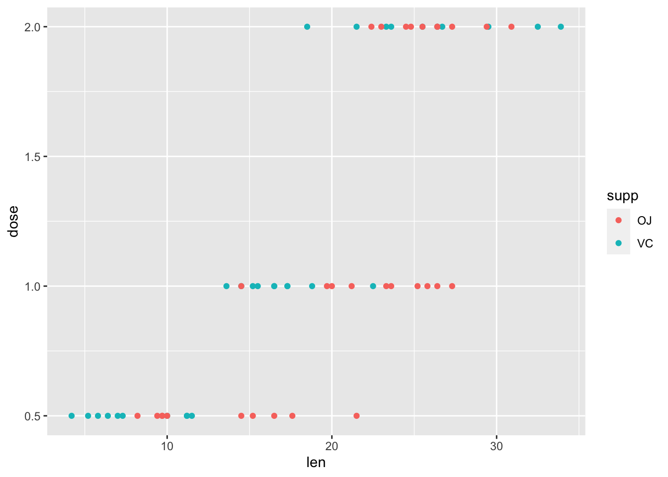
Based on the plot, we can see len seems increasing when dose increases.
根据该图,我们可以看到 dose 增加时 len 也增加。
We can't find a clear relationship between len and supp .
我们无法找到 len 和 supp 之间的明确关系。
Let's try a boxplot.
再尝试一下箱线图。
ggplot(data = ToothGrowth) + geom_boxplot(mapping = aes(x = supp, y = len)) |
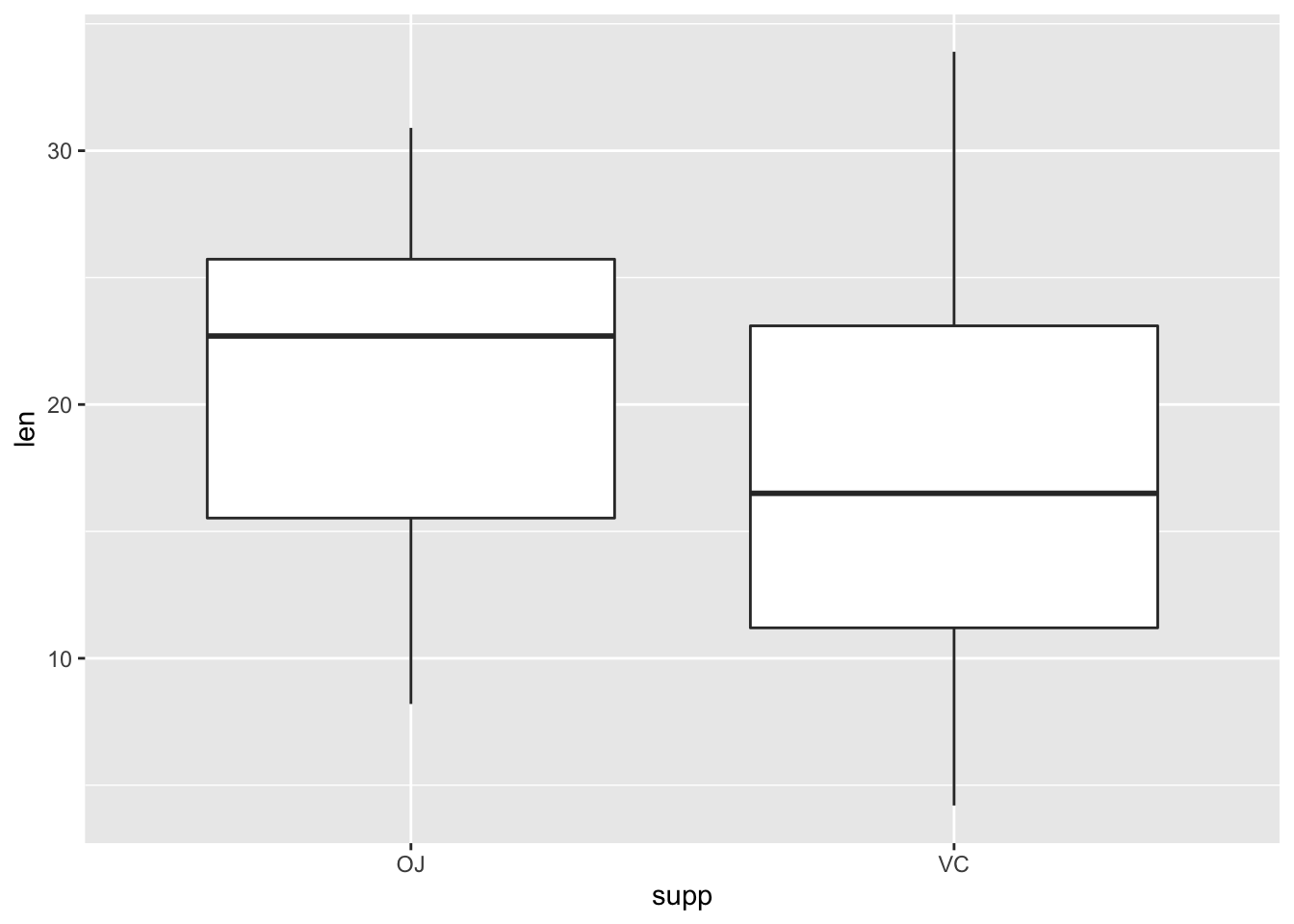
Based on the graph, we may have the conjecture the means and variances of len are different between these two supp .
根据该图,我们可以推测这两个样本 supp 的 len 的均值和方差是不同的。
Let's do an F test first. Consider .
先做一个 F 检验。考虑 。
var.test(len ~ supp, data = ToothGrowth) |
    F test to compare two variances

data:  len by supp
F = 0.6386, num df = 29, denom df = 29, p-value = 0.2331
alternative hypothesis: true ratio of variances is not equal to 1
95 percent confidence interval:
 0.3039488 1.3416857
sample estimates:
ratio of variances
         0.6385951
# In-class Exercise
Will you reject or not? Why?
你会拒绝 吗?或不拒绝?为什么?Based on the result of F test, do a hypothesis testing for the mean of
lenbetween twosupp. What is your conclusion?
根据 F 检验的结果,这两个样本supp的len均值进行假设检验。你的结论是什么?
We should not reject as p value is larger than 0.05.
t.test(len~supp, data = ToothGrowth,var.equal = TRUE) |
    Two Sample t-test

data:  len by supp
t = 1.9153, df = 58, p-value = 0.06039
alternative hypothesis: true difference in means is not equal to 0
95 percent confidence interval:
 -0.1670064  7.5670064
sample estimates:
mean in group OJ mean in group VC
        20.66333         16.96333
We should not reject .
# Summary of hypothesis testing 假设检验总结
- Three elements of a test: hypotheses, test statistic, and critical region
检验的三个要素:假设、检验统计量和临界区 - In practice, check assumptions to know which test to use (i.e., which distribution to reference)
在实践中,检查假设以了解使用哪种测试(即参考哪个分布) - We learned about: one- and two-population location and scale problems, in continuous setting, and proportion in discrete setting
了解了:连续环境下的单总体和双总体区位和规模问题,离散环境下的比例问题
# References
- Probability & Statistics for Engineers & Scientist, 9th Edition, Ronald E. Walpole, Raymond H. Myers, Sharon L. Myers, Keying Ye, Prentice Hall