# Objective

• Multiple linear regression
  多元线性回归
• Basic R and Python command to run a multiple linear regression model
  基本的 R 和 Python 命令运行一个多元线性回归模型
• Subset Selection (Forward/Backward Selection)
  子集选择 (向前 / 向后选择)

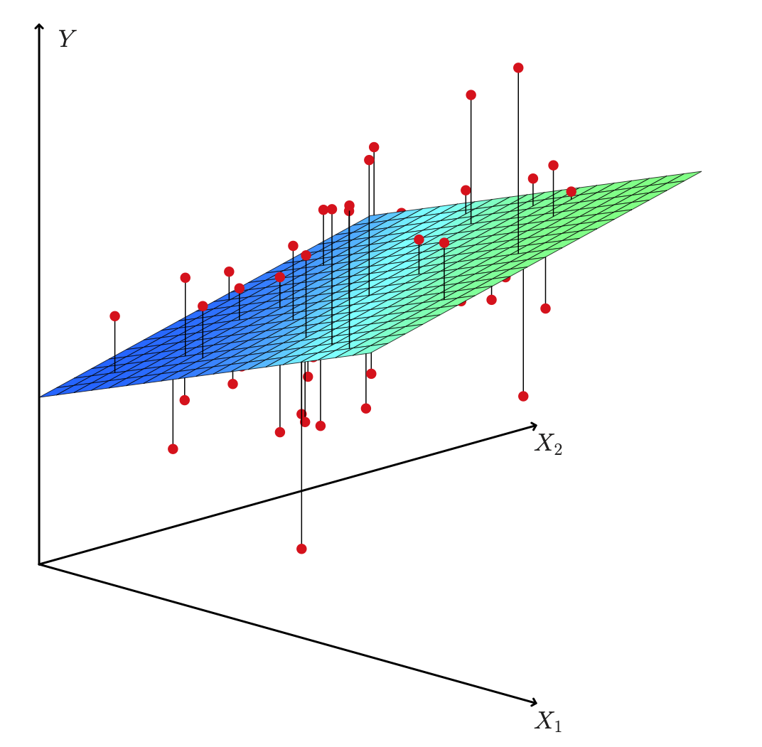
# Multiple Linear Regression

• Predict a quantitative $Y$ by more than one predictor variable $X_i$
  通过多个预测变量$X_i$ 预测定量$Y$

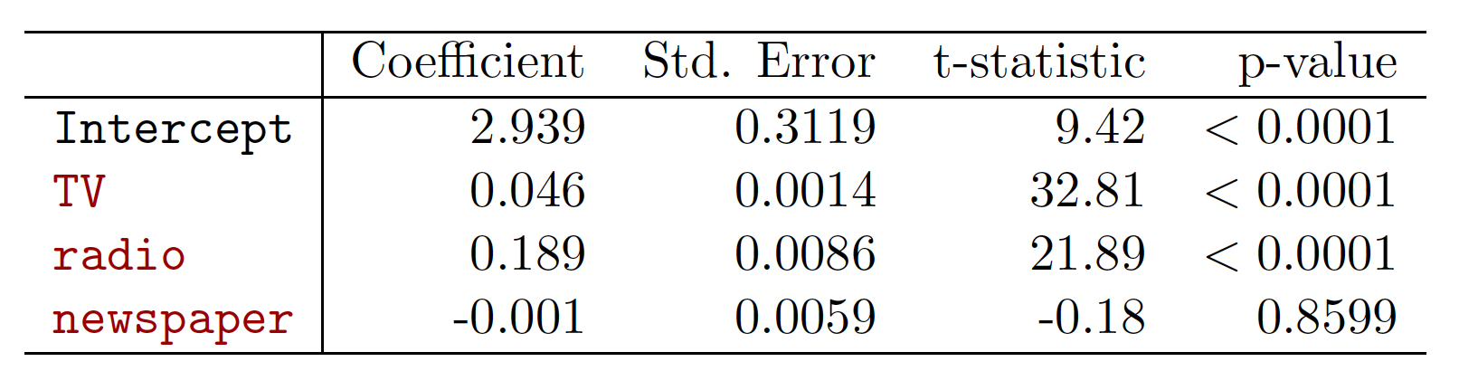
  $$Y \approx \beta_0+\beta_1 X_1+ \beta_2X_2 + \ldots + \beta_pX_p.$$

• Advertising Example:

$$sales \approx \beta_0+\beta_1\times TV + \beta_2\times radio + \beta_3 \times newspaper$$

• We interpret $\beta_j$ as the average effect on $Y$ of a one unit increase in $X_j$, holding all other predictors fixed.
  $\beta_j$ 指保持所有其他预测变量不变，$X_j$ 增加一个单位对$Y$ 的平均影响

# How to estimate the coefficients 如何估计系数

Let $\hat{y}_i = \hat\beta_0+\hat\beta_1x_i+ \hat\beta_2x_2 + \ldots + \hat\beta_px_p$ be the prediction for $Y$ based on the $i$th value of $X$.
... 是基于$X$ 的第$i$ 个值，对$Y$ 的预测。

$e_i = y_i-\hat{y}_i$ represents the $i$th residual.
... 表示第$i$ 个残差。

Residual Sum of Squares RSS 残差平方和

$$\text{RSS} = \sum_{i=1}^n e_i^2 = \sum_{i=1}^n(y_i-\hat{y}_i)^2 = \sum_{i=1}^n(y_i-(\hat\beta_0+\hat\beta_1x_i+ \hat\beta_2x_2 + \ldots + \hat\beta_px_p))^2.$$

The values $\hat\beta_0,\hat\beta_1,\ldots,\hat\beta_p$ that minimize RSS are the multiple least squares regression coefficient estimates.
最小化 RSS 的这些值，是多重最小二乘回归系数估计值。

Advertising Example

# Is at least one predictor useful? 至少有一个预测变量是可用吗？

Question: is there a relationship between the Response and Predictor?
响应变量和预测变量之间有关系吗？

• Multiple case: $p$ predictors; we need to ask whether all of the regression coefficients are zero: $\beta_1=\dots=\beta_p=0$?
  多种情况:$p$ 个预测变量；需要考虑是否所有的回归系数都是零: $\beta_1=\dots=\beta_p=0$?

  • Hypothesis test: $H_0:\beta_1=\dots=\beta_p=0$ vs. $H_1:$ at least one $\beta_i\neq 0$. 假设检验
  • Which statistic? 哪个统计量？ $$ F= \frac {(TSS-RSS)/p}{RSS/(n-p-1)}. $$
    • TSS = total sum of squares 总平方和
      $\sum_{i=1}^n(y_i-\bar y)^2$ where $\bar y = \frac{1}{n}\sum_{i=1}^ny_i$
    • RSS = residual sum of squares 残差平方和
      $\sum_{i=1}^n(y_i-\hat y_i)^2$

• when there is no relationship between the response and predictors, one would expect the F-statistic to take on a value close to 1. [this can be proved via expected values]
  当响应变量和预测变量之间没有关系时，人们会期望 F 统计量取值接近 1。 [这可以通过期望值来证明]

• else $>1$.
  或者 $>1$。

Revisiting Advertising Example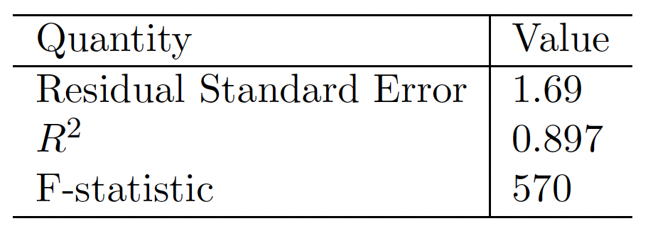

# Multiple linear Regression in R R 中的多元线性回归

• Include the package and data; Let's split the data set into two parts AutoTraining and AutoTest
  包括包和数据；将数据集分成两部分， AutoTraining 和 AutoTest

library(ISLR)

data(Auto)

i <- sample(2, nrow(Auto), replace=TRUE, prob=c(0.8, 0.2))

AutoTraining <- Auto[i==1,]

AutoTest <- Auto[i==2,]

• Produce a scatterplot matrix which includes all of the variables in the data set.
  生成一个散点图矩阵，其中包括数据集中的所有变量。

pairs(AutoTraining[,1:8],lower.panel = NULL)

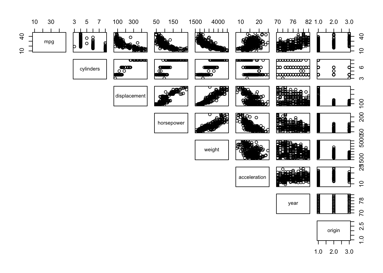
What are we looking at? (Read the help page on pairs .)

• Compute the matrix of correlations between the variables using the function cor() . You will need to exclude the name variable, which is qualitative.
  使用函数 cor() 计算变量之间的相关性矩阵。您需要排除 name 变量，它是定性的。

cor(subset(AutoTraining, select=-name))

                    mpg  cylinders displacement horsepower     weight
mpg           1.0000000 -0.7835984   -0.8093361 -0.7756140 -0.8322683
cylinders    -0.7835984  1.0000000    0.9488134  0.8482233  0.8973357
displacement -0.8093361  0.9488134    1.0000000  0.8980871  0.9312435
horsepower   -0.7756140  0.8482233    0.8980871  1.0000000  0.8594881
weight       -0.8322683  0.8973357    0.9312435  0.8594881  1.0000000
acceleration  0.4073567 -0.5128548   -0.5471046 -0.6944759 -0.4124139
year          0.5741327 -0.3239422   -0.3513303 -0.3997054 -0.2927119
origin        0.5750312 -0.5547678   -0.6012353 -0.4486185 -0.5745900
             acceleration       year     origin
mpg             0.4073567  0.5741327  0.5750312
cylinders      -0.5128548 -0.3239422 -0.5547678
displacement   -0.5471046 -0.3513303 -0.6012353
horsepower     -0.6944759 -0.3997054 -0.4486185
weight         -0.4124139 -0.2927119 -0.5745900
acceleration    1.0000000  0.2665451  0.2120587
year            0.2665451  1.0000000  0.1861288
origin          0.2120587  0.1861288  1.0000000

• Use the lm() function to perform a multiple linear regression with mpg as the response and all other variables except name as the predictors. Print results.
  使用 lm() 函数执行多元线性回归，以 mpg 作为响应变量，以除名称之外的所有其他变量作为预测变量。打印结果。

fitlm <- lm(mpg~., data=AutoTraining[,1:8])

summary(fitlm)

Call:
lm(formula = mpg ~ ., data = AutoTraining[, 1:8])

Residuals:
    Min      1Q  Median      3Q     Max 
-9.0922 -1.9274 -0.0704  1.7586 12.6889 

Coefficients:
               Estimate Std. Error t value Pr(>|t|)    
(Intercept)  -1.632e+01  5.187e+00  -3.147  0.00181 ** 
cylinders    -6.026e-01  3.523e-01  -1.711  0.08818 .  
displacement  1.596e-02  8.159e-03   1.956  0.05136 .  
horsepower   -2.099e-02  1.550e-02  -1.354  0.17677    
weight       -5.853e-03  7.214e-04  -8.114 1.26e-14 ***
acceleration -7.949e-03  1.094e-01  -0.073  0.94212    
year          7.548e-01  5.689e-02  13.268  < 2e-16 ***
origin        1.583e+00  3.193e-01   4.957 1.20e-06 ***
---
Signif. codes:  0 '***' 0.001 '**' 0.01 '*' 0.05 '.' 0.1 ' ' 1

Residual standard error: 3.322 on 301 degrees of freedom
Multiple R-squared:  0.8275,    Adjusted R-squared:  0.8235 
F-statistic: 206.3 on 7 and 301 DF,  p-value: < 2.2e-16

Let's refer to the output in this last code chunk:
最后一个代码块中的输出:

• Is there a relationship between the predictors and the response?
  预测变量和响应变量之间是否存在关系？

  • There is a relationship between predictors and response.
    预测变量和响应变量之间存在关系。

• Which predictors appear to have a statistically significant relationship to the response?
  哪些预测变量似乎与响应变量有统计学上的显著关系？

  • weight , year , origin and displacement have statistically significant relationships
    weight , year , origin and displacement 有统计上的显著关系

• What does the coefficient for the year variable suggest?
  year 变量的系数意味着什么？

  • r fitlm$coefficients[7] 0.7547858 coefficient for year suggests that later model year cars have better (higher) mpg .
    year 的系数 0.7547858 表明较晚的车型年拥有更好 (更高) 的 mpg 。

• Use the plot() function to produce diagnostic plots of the linear regression fit.
  使用 plot() 函数生成线性回归拟合的诊断图。

par(mfrow=c(2,2))

plot(fitlm)

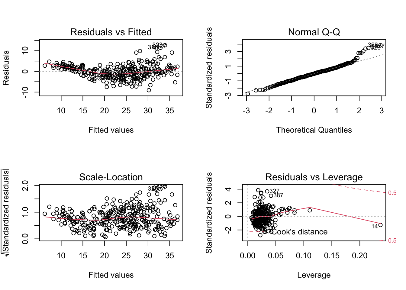
• Comment on any problems you see with the fit. Do the residual plots suggest any unusually large outliers?
  对你认为合适的任何问题进行评论。残差图是否暗示了任何异常大的异常值？
  • There is evidence of non-linearity
    有非线性的证据

First you have to make a new data frame object which will contain the new point:
首先，必须创建一个包含新点的新数据框对象:

ypred <-predict(object = fitlm, newdata = AutoTest[,1:8])

summary(ypred)

   Min. 1st Qu.  Median    Mean 3rd Qu.    Max. 
  6.557  20.725  25.966  24.798  30.416  36.330 

To evaluate the mean absolute error (MAE) and mean squared error (MSE), we can install MLmetric package.
为了评估平均绝对误差 MAE 和均方误差 MSE ，我们可以安装 MLmetric 包。

$$MAE = \frac{\sum_{i=1}^n |y_i-\hat{y}_i|}{n}, \qquad MSE = \frac{\sum_{i=1}^n (y_i-\hat{y}_i)^2}{n}.$$

library(MLmetrics)

Attaching package: 'MLmetrics'

The following object is masked from 'package:base':

    Recall

MAE(y_pred = ypred, y_true = AutoTest$mpg)

[1] 2.729826

MSE(y_pred = ypred, y_true = AutoTest$mpg)

[1] 11.7072

# Multiple linear regression in Python

library(reticulate)

# import the necessary packages

import pandas as pd

import numpy as np

import statsmodels.api as sm #py_install("statsmodels")

Let's read the dataset first.

# Read the data set from the website of our textbook

auto = pd.read_csv('https://www.statlearning.com/s/Auto.csv')

# Here I dropped the records with horsepower = ?

auto = auto.drop(labels=[32,126,330,336,354], axis=0)

• Let's split the data set into two parts auto_training and auto_testing
  把数据集分成两部分 auto_training 和 auto_testing

auto_training = auto.sample(frac = 0.8)

auto_testing = auto.drop(auto_training.index)

# choose the predictor

X = pd.DataFrame(auto_training[['cylinders','displacement','horsepower','weight','acceleration','year','origin']])

# choose the response

y = auto_training[['mpg']]

# add a constant to the predictor

X = sm.add_constant(X)

# OLS stands for “Ordinary Least Squares”

# `horsepower` consider as a object, so I use astype to convert it to numeric

model01 = sm.OLS(y, X.astype(float)).fit()

# To obtain the results of the regression model, run the `summary()` command on the model

model01.summary()

OLS Regression Results
Dep. Variable:	mpg	R-squared:	0.818
Model:	OLS	Adj. R-squared:	0.814
Method:	Least Squares	F-statistic:	196.8
Date:	Mon, 08 Nov 2021	Prob (F-statistic):	2.82e-109
Time:	11:22:03	Log-Likelihood:	-827.06
No. Observations:	314	AIC:	1670.
Df Residuals:	306	BIC:	1700.
Df Model:	7		
Covariance Type:	nonrobust		
coef	std err	t	P>|t|	[0.025	0.975]
const	-16.3943	5.336	-3.073	0.002	-26.893	-5.895
cylinders	-0.5409	0.372	-1.455	0.147	-1.273	0.191
displacement	0.0181	0.008	2.148	0.032	0.002	0.035
horsepower	-0.0159	0.016	-0.984	0.326	-0.048	0.016
weight	-0.0063	0.001	-8.425	0.000	-0.008	-0.005
acceleration	0.1146	0.112	1.021	0.308	-0.106	0.335
year	0.7352	0.059	12.508	0.000	0.620	0.851
origin	1.3712	0.325	4.220	0.000	0.732	2.011
Omnibus:	26.087	Durbin-Watson:	2.126
Prob(Omnibus):	0.000	Jarque-Bera (JB):	42.721
Skew:	0.524	Prob(JB):	5.29e-10
Kurtosis:	4.472	Cond. No.	8.64e+04

Notes:
[1] Standard Errors assume that the covariance matrix of the errors is correctly specified.
[2] The condition number is large, 8.64e+04. This might indicate that there are
strong multicollinearity or other numerical problems.

• Evaluate the prediction error 评估预测误差

X_test = pd.DataFrame(auto_testing[['cylinders','displacement','horsepower','weight','acceleration','year','origin']])

X_test = sm.add_constant(X_test.astype(float))

ypred = model01.predict(X_test)

from sklearn import metrics #py_install("scikit-learn")

# calculate MAE, MSE, RMSE

print(metrics.mean_absolute_error(y_true = auto_testing[['mpg']], y_pred = ypred))

2.3932979890707395

print(metrics.mean_squared_error(y_true = auto_testing[['mpg']], y_pred = ypred))

8.928246249434233

# How to choose the important variables? 重要的变量如何选择？

The most direct approach is called all subsets or best subsets regression: we compute the least squares fit for all possible subsets and then choose between them based on some criterion that balances training error with model size.
最直接的方法称为所有子集或最佳子集回归：我们计算所有可能子集的最小二乘拟合，然后根据平衡训练误差和模型大小的标准在它们之间进行选择。

However, we often can't examine all possible models, since they are $2^p$ of them; for example when $p = 40$ there are over a billion models!
然而，我们往往不能考察所有可能的模型，因为它们是其中的$2^p$；例如，当$p = 40$ 时，有超过 10 亿个模型！

Instead we need an automated approach that searches through a subset of them.
相反，我们需要一种自动化的方法来搜索它们的子集。

We discuss two commonly use approaches next.
接下来我们讨论两种常用的方法

# Forward Selection 预选

• Begin with the null model --- a model that contains an
  intercept but no predictors.
  从空模型开始 - 一个包含截距但没有预测变量的模型。
• Fit $p$ simple linear regressions and add to the null model the variable that results in the lowest RSS.
  拟合$p$ 简单线性回归，并在空模型中添加导致最低 RSS 的变量。
• Add to that model the variable that results in the lowest RSS amongst all two-variable models.
  向该模型中添加导致所有双变量模型中最低 RSS 的变量。
• Continue until some stopping rule is satisfied, for example when all remaining variables have a p-value above some threshold.
  继续，直到满足某个停止规则，例如当所有剩余变量的 p 值高于某个阈值时。

Revisit Auto data set

To run stepwise regression, you first need to install and open the MASS package.
要运行逐步回归，你首先需要安装并打开 MASS 包。

library(MASS)

# Create a null model 

# 创建一个空模型

intercept_only <- lm(mpg ~ 1, data=AutoTraining[,1:8])

# Create a full model

# 创建一个完整的模型

all <- lm(mpg~., data=AutoTraining[,1:8])

# perform forward step-wise regression

# 执行向前逐步回归

forward <- stepAIC (intercept_only, direction='forward',scope = formula(all))

Start:  AIC=1278.89
mpg ~ 1

               Df Sum of Sq     RSS     AIC
+ weight        1   13339.3  5918.5  916.32
+ displacement  1   12614.4  6643.5  952.03
+ cylinders     1   11824.8  7433.0  986.73
+ horsepower    1   11585.1  7672.8  996.54
+ origin        1    6367.8 12890.0 1156.84
+ year          1    6347.9 12909.9 1157.31
+ acceleration  1    3195.6 16062.2 1224.82
<none>                      19257.9 1278.89

Step:  AIC=916.32
mpg ~ weight

               Df Sum of Sq    RSS    AIC
+ year          1   2300.91 3617.6 766.21
+ origin        1    269.49 5649.0 903.92
+ horsepower    1    267.91 5650.6 904.01
+ displacement  1    170.54 5748.0 909.29
+ cylinders     1    133.70 5784.8 911.26
+ acceleration  1     95.40 5823.1 913.30
<none>                      5918.5 916.32

Step:  AIC=766.21
mpg ~ weight + year

               Df Sum of Sq    RSS    AIC
+ origin        1   234.723 3382.9 747.48
<none>                      3617.6 766.21
+ cylinders     1    21.592 3596.0 766.36
+ displacement  1     5.188 3612.4 767.77
+ horsepower    1     3.692 3613.9 767.89
+ acceleration  1     3.104 3614.5 767.94

Step:  AIC=747.48
mpg ~ weight + year + origin

               Df Sum of Sq    RSS    AIC
<none>                      3382.9 747.48
+ horsepower    1   14.4372 3368.4 748.16
+ cylinders     1    9.2172 3373.7 748.64
+ acceleration  1    5.4873 3377.4 748.98
+ displacement  1    1.3438 3381.5 749.36

# view results of backward stepwise regression

# 后向逐步回归的视图结果

forward$anova

Stepwise Model Path 
Analysis of Deviance Table

Initial Model:
mpg ~ 1

Final Model:
mpg ~ weight + year + origin

      Step Df   Deviance Resid. Df Resid. Dev       AIC
1                              308  19257.851 1278.8908
2 + weight  1 13339.3470       307   5918.504  916.3218
3   + year  1  2300.9100       306   3617.594  766.2090
4 + origin  1   234.7231       305   3382.871  747.4799

# view final model

# 查看最终模型

summary(forward)

Call:
lm(formula = mpg ~ weight + year + origin, data = AutoTraining[, 
    1:8])

Residuals:
    Min      1Q  Median      3Q     Max 
-8.7628 -2.0335 -0.0755  1.6494 12.7616 

Coefficients:
              Estimate Std. Error t value Pr(>|t|)    
(Intercept) -19.206296   4.424806  -4.341 1.94e-05 ***
weight       -0.006014   0.000279 -21.558  < 2e-16 ***
year          0.770039   0.053872  14.294  < 2e-16 ***
origin        1.376791   0.299284   4.600 6.19e-06 ***
---
Signif. codes:  0 '***' 0.001 '**' 0.01 '*' 0.05 '.' 0.1 ' ' 1

Residual standard error: 3.33 on 305 degrees of freedom
Multiple R-squared:  0.8243,    Adjusted R-squared:  0.8226 
F-statistic: 477.1 on 3 and 305 DF,  p-value: < 2.2e-16

Check the MAE and MSE

ypred_forward <-predict(object = forward, newdata = AutoTest[,1:8])

MAE(y_pred = ypred_forward, y_true = AutoTest$mpg)

[1] 2.684931

MSE(y_pred = ypred_forward, y_true = AutoTest$mpg)

[1] 11.89915

# Backward Selection

• Start with all variables in the model.
  从模型中的所有变量开始。
• Remove the variable with the largest p-value --- that is, the variable that is the least statistically significant.
  去掉 p 值最大的变量，也就是统计意义最小的变量。
• The new $(p-1)$-variable model is fit, and the variable with the largest p-value is removed.
  新的$(p-1)$- 变量模型被拟合，具有最大 p 值的变量被移除。
• Continue until a stopping rule is reached. For instance, we may stop when all remaining variables have a significant p-value defined by some significance threshold.
  继续，直到达到停止规则。例如，当所有剩余变量都具有由某个显著性阈值定义的显著 p 值时，我们可以停止。

Similarly, we use the same function stepAIC from MASS package
类似地，我们从 MASS 包中使用相同的函数 stepAIC

backward <- stepAIC (all, direction='backward')

Start:  AIC=749.85
mpg ~ cylinders + displacement + horsepower + weight + acceleration + 
    year + origin

               Df Sum of Sq    RSS    AIC
- acceleration  1      0.06 3321.9 747.86
- horsepower    1     20.23 3342.1 749.73
<none>                      3321.8 749.85
- cylinders     1     32.29 3354.1 750.84
- displacement  1     42.23 3364.1 751.76
- origin        1    271.17 3593.0 772.10
- weight        1    726.49 4048.3 808.97
- year          1   1942.80 5264.6 890.15

Step:  AIC=747.86
mpg ~ cylinders + displacement + horsepower + weight + year + 
    origin

               Df Sum of Sq    RSS    AIC
<none>                      3321.9 747.86
- horsepower    1     31.21 3353.1 748.75
- cylinders     1     32.24 3354.1 748.84
- displacement  1     43.00 3364.9 749.83
- origin        1    271.11 3593.0 770.10
- weight        1    965.95 4287.8 824.73
- year          1   1964.66 5286.6 889.43

backward$anova

Stepwise Model Path 
Analysis of Deviance Table

Initial Model:
mpg ~ cylinders + displacement + horsepower + weight + acceleration + 
    year + origin

Final Model:
mpg ~ cylinders + displacement + horsepower + weight + year + 
    origin

            Step Df   Deviance Resid. Df Resid. Dev      AIC
1                                    301   3321.840 749.8543
2 - acceleration  1 0.05826504       302   3321.898 747.8597

summary(backward)

Call:
lm(formula = mpg ~ cylinders + displacement + horsepower + weight + 
    year + origin, data = AutoTraining[, 1:8])

Residuals:
    Min      1Q  Median      3Q     Max 
-9.0858 -1.9311 -0.0626  1.7232 12.6835 

Coefficients:
               Estimate Std. Error t value Pr(>|t|)    
(Intercept)  -1.650e+01  4.609e+00  -3.579 0.000402 ***
cylinders    -6.011e-01  3.511e-01  -1.712 0.087905 .  
displacement  1.602e-02  8.103e-03   1.977 0.048929 *  
horsepower   -2.028e-02  1.204e-02  -1.684 0.093144 .  
weight       -5.879e-03  6.274e-04  -9.371  < 2e-16 ***
year          7.552e-01  5.651e-02  13.365  < 2e-16 ***
origin        1.582e+00  3.187e-01   4.965 1.15e-06 ***
---
Signif. codes:  0 '***' 0.001 '**' 0.01 '*' 0.05 '.' 0.1 ' ' 1

Residual standard error: 3.317 on 302 degrees of freedom
Multiple R-squared:  0.8275,    Adjusted R-squared:  0.8241 
F-statistic: 241.5 on 6 and 302 DF,  p-value: < 2.2e-16

#Get MAE and MSE

ypred_backward <-predict(object = backward, newdata = AutoTest[,1:8])

MAE(y_pred = ypred_backward, y_true = AutoTest$mpg)

[1] 2.728393

MSE(y_pred = ypred_backward, y_true = AutoTest$mpg)

[1] 11.68725

# Both-direction stepwise selection

We can also do both-direction stepwise selection
我们也可以做双向逐步选择

both <- stepAIC (intercept_only, direction='both',scope = formula(all),trace = 0)

both$anova

Stepwise Model Path 
Analysis of Deviance Table

Initial Model:
mpg ~ 1

Final Model:
mpg ~ weight + year + origin

      Step Df   Deviance Resid. Df Resid. Dev       AIC
1                              308  19257.851 1278.8908
2 + weight  1 13339.3470       307   5918.504  916.3218
3   + year  1  2300.9100       306   3617.594  766.2090
4 + origin  1   234.7231       305   3382.871  747.4799

summary(both)

Call:
lm(formula = mpg ~ weight + year + origin, data = AutoTraining[, 
    1:8])

Residuals:
    Min      1Q  Median      3Q     Max 
-8.7628 -2.0335 -0.0755  1.6494 12.7616 

Coefficients:
              Estimate Std. Error t value Pr(>|t|)    
(Intercept) -19.206296   4.424806  -4.341 1.94e-05 ***
weight       -0.006014   0.000279 -21.558  < 2e-16 ***
year          0.770039   0.053872  14.294  < 2e-16 ***
origin        1.376791   0.299284   4.600 6.19e-06 ***
---
Signif. codes:  0 '***' 0.001 '**' 0.01 '*' 0.05 '.' 0.1 ' ' 1

Residual standard error: 3.33 on 305 degrees of freedom
Multiple R-squared:  0.8243,    Adjusted R-squared:  0.8226 
F-statistic: 477.1 on 3 and 305 DF,  p-value: < 2.2e-16

#Get MAE and MSE

ypred_both <-predict(object = both, newdata = AutoTest[,1:8])

MAE(y_pred = ypred_both, y_true = AutoTest$mpg)

[1] 2.684931

MSE(y_pred = ypred_both, y_true = AutoTest$mpg)

[1] 11.89915

# Reference

1. Chapter 3 of the textbook Gareth James, Daniela Witten, Trevor Hastie and Robert Tibshirani, An Introduction to Statistical Learning: with Applications in R.

2. Chapter 11 of the textbook Chantal D. Larose
   and Daniel T. Larose Data Science Using Python and R.

3. Part of this lecture notes are extracted from Prof. Sonja Petrovic ITMD/ITMS 514 lecture notes.