# Outline
- An Overview of Statistical Learning
统计学习概述 - What is Statistical Learning?
什么是统计学习? - Assessing Model Accuracy
评估模型精度
# An Overview of Statistical Learning
# Introduction to Statistical Learning
- Statistical learning 统计学习
- refers to a vast set of tools for understanding data.
指用于理解数据的大量工具。
These tools can be classified as supervised or unsupervised.
这些工具可分为有监督的和无监督的。 - Supervised learning 监督式学习
- building a statistical model for predicting, or estimating, an output based on one or more inputs.
建立一个统计模型来预测或估计一个或多个输入。 - Unsupervised learning 无监督学习
- no supervising output; find relationships and structure from such data.
没有监督输出;从这些数据中找到关系和结构。
# Statistical Learning Problems 统计学习问题
Identify the numbers in a handwritten zip code
识别手写邮政编码中的数字
Establish the relationship between salary and demographic variables in population survey data
在人口调查数据中建立工资和人口统计变量之间的关系
Predict whether the index will increase or decrease on a given day using the past 5 days percentage changes in the index
使用过去 5 天的指数变化百分比来预测某一天的指数是否会增加或减少
Understand which types of customers are similar to each other by grouping individuals according to their observed characteristics
根据观察到的顾客特征对他们进行分组,从而了解哪些类型的顾客是相似的


# Supervised Learning Problem 监督学习问题
- Outcome measurement (also called dependent variable, response, target).
结果测量 (也称因变量、响应、目标)。 - Vector of m predictor measurements (also called independent variables, inputs, attributes, features).
向量 m 预测值的测量 (也称为自变量,输入,属性,特征)。 - In the regression problem, is quantitative (e.g price, blood pressure).
在 回归 问题中,Y 是定量的 (例如价格、血压)。 - In the classification problem, takes values in a finite, unordered set (survived/died, digit 0-9, cancer class of tissue sample).
在 分类 问题中, 在有限的无序集合中取值 (存活 / 死亡,数字 0-9,组织样本的癌症类别)。 - We have training data : These are observations (examples, instances) of these measurements.
我们有训练数据:这些是测量的观察结果 (示例,实例)
On the basis of the training data we would like to:
在训练数据的基础上,我们希望:
- Accurately predict unseen test cases.
准确预测看不见的测试用例。 - Understand which inputs affect the outcome, and how.
了解哪些投入会影响结果,以及如何影响结果。 - Assess the quality of our predictions and inferences.
评估我们的预测和推论的质量。
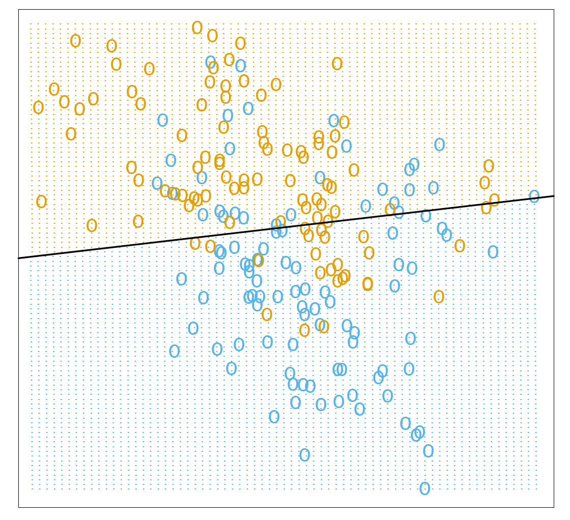
# A Linear Model and Least Squares Example 线性模型和最小二乘示例
An example of the linear model in a classification context.
分类环境中的线性模型示例。
Two predicted classes are separated by the decision boundary .
决策边界将两个预测类分开
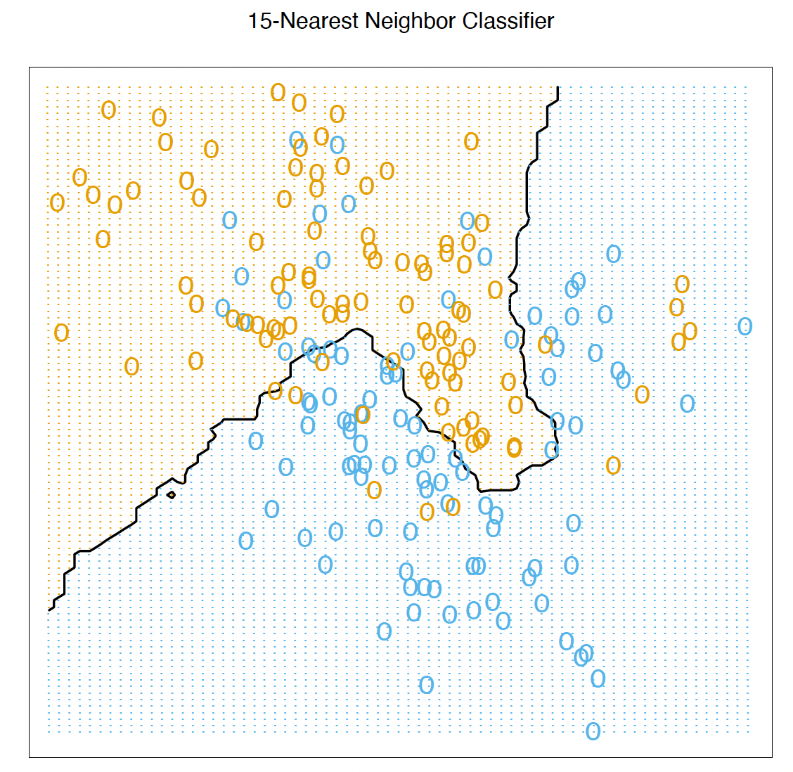
# K-Nearest Neighbor Example K - 最近邻示例
The same classification example and then fit by 15-nearest-neighbor averaging.
The predicted class is chosen by majority vote amongst the 15nearest neighbors.
相同的分类实例,然后通过 15 近邻平均进行拟合。
预测的类别是从 15 个最近的邻居中以多数票选出的。
# Unsupervised Learning Problem 无监督学习问题
- No outcome variable, just a set of predictors (features) measured on a set of samples.
没有结果变量,只是在一组样本上测量的一组预测因子 (特征)。 - objective is more fuzzy — find groups of samples that behave similarly, find features that behave similarly, find linear combinations of features with the most variation.
目标更加模糊 —— 找出行为相似的样本组,找出行为相似的特征,找出变化最大的特征线性组合。 - diffcult to know how well your are doing.
很难知道你做得怎么样。 - different from supervised learning, but can be useful as a pre-processing step for supervised learning.
不同于监督式学习,但可作为监督式学习的预处理步骤。
# Clustering Example with Three Groups 三组聚类示例
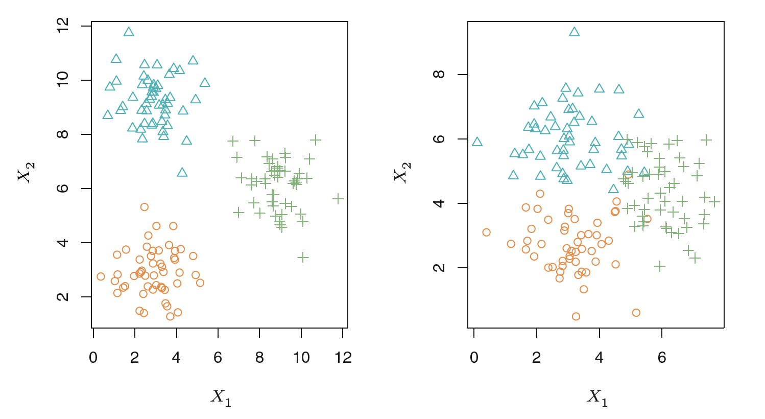
Left: The three groups are well-separated. In this setting, a clustering approach should successfully identify the three groups.
左图:三组分离得很好。在这种情况下,聚类方法应该成功地识别这三个组。
Right: There is some overlap among the groups.
右图:各组之间有一些重叠。
Now the clustering task is more challenging.
现在集群任务更具挑战性。
# Real Problems
- Spam filter
垃圾邮件过滤器 - Malware classification
恶意软件分类 - Anomaly detection problems such as fraud detection
异常检测问题,如欺诈检测 - Recommendation system
推荐系统 - Identifying fake news
识别假新闻
One example with Iris Data: Clustering for Iris
# Statistical Learning VS Machine Learning
- Machine learning arose as a subeld of Articial Intelligence.
机器学习是人工智能的一个分支。 - Statistical learning arose as a subeld of Statistics.
统计学习是作为统计学的一个分支出现的。 - There is much overlap — both fields focus on supervised and unsupervised problems:
有很多重叠 —— 两个领域都关注监督和非监督问题:- Machine learning has a greater emphasis on large scale applications and prediction accuracy.
机器学习更强调大规模应用和预测准确性。 - Statistical learning emphasizes models and their interpretability, and precision and uncertainty.
统计学习强调模型及其可解释性、精确性和不确定性。
But the distinction has become more and more blurred, and there is a great deal of cross-fertilization.
但是这种区别已经变得越来越模糊,并且存在大量的交叉现象。
- Machine learning has a greater emphasis on large scale applications and prediction accuracy.
# What is Statistical Learning?
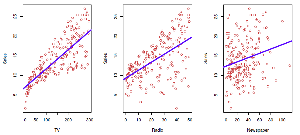
Shown are Sales vs TV , Radio and Newspaper , with a blue linear-regression line fit separately to each.
图中显示的是 Sales 与电视、广播和报纸,蓝色线性回归线分别与它们相吻合。
Can we predict Sales using these three?
我们能用这三个预测销售额吗?
Perhaps we can do better using a model
也许我们可以用模型做得更好
Here Sales is a response or target that we wish to predict. We generically refer to the response as .
在这里, Sales 是我们希望预测的响应或目标。我们一般把它称为 。
TV is a feature, or input, or predictor; we name it : Likewise name Radio as ; and so on. We can refer to the input vector collectively asTV 是一个特征,或输入,或预测;我们把它命名为: 同样把 Radio 命名为;等等。我们可以将 输入向量 统称为
Now we write our model as ; where captures measurement errors and other discrepancies.
现在我们把模型写成 ; 捕捉测量误差和其他差异。
More generally, suppose that we observe a quantitative response and different predictors, : Let , which can be written in the very general form .
简单来说,假设我们观察到一个定量响应 ,以及 个不同的预测因子, 。 ,可以用 的常规形式来表示。
is a random error term, which is independent of and has mean zero.
是一个随机误差项,与 无关,均值为零。
In this formulation, represents the systematic information that provides about .
在这个公式中, 代表了 提供的关于 的系统信息。
Another Example
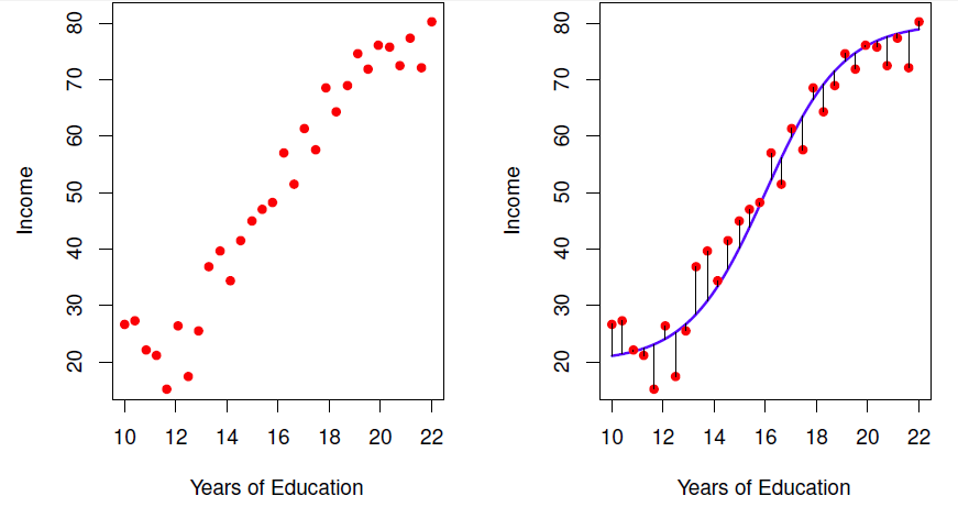
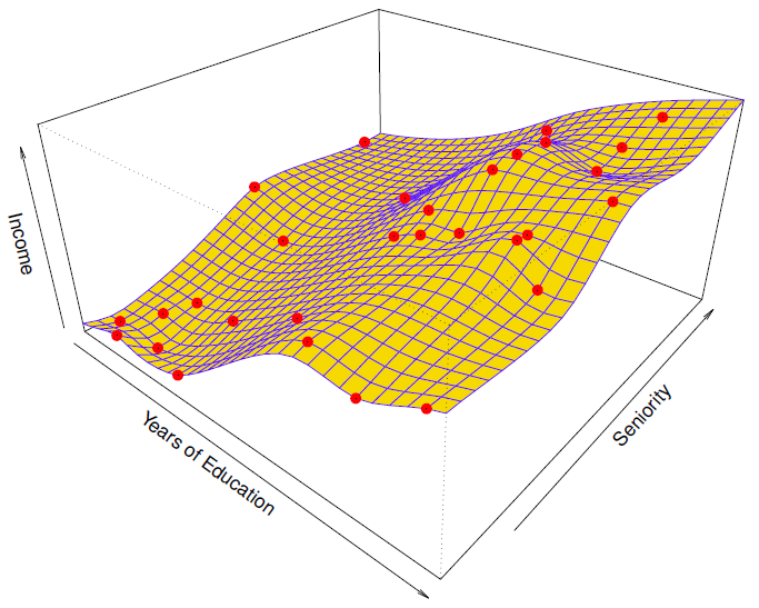
Figure: Left: The red dots are the observed values of income (in tens of thousands of dollars) and years of education for 30 individuals.
左图:红点是观察到的 30 个人的收入 (以万美元计) 和教育年限的数值。
Right: The blue curve represents the true underlying relationship between income and years of education, which is generally unknown (but is known in this case because the data were simulated).
右图:蓝色曲线代表收入和教育年限之间的真实潜在关系,这通常是未知的 (但在本例中是已知的,因为数据是模拟的)。
# What is good for?
- With a good we can make predictions of at new points .
- We can understand which components of are important in explaining , and which are irrelevant.
我们可以理解 中的哪些成分对解释 是重要的,哪些是无关的。
e.g.SeniorityandYears of Educationhave a big impact onIncome, butMarital Statusdoes not.
例如:“资历” 和 “受教育年限” 对 “收入” 有很大影响,但 “婚姻状况” 没有。 - Depending on the complexity of , we may be able to understand how each component of affects .
根据 的复杂度,我们可以理解 的每个分量 如何影响。
# Is There an Ideal ?
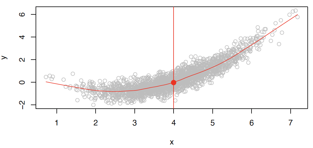
In particular, what is a good value for at any selected value of , say ?
在任意选定的 值 (比如) 上的值是多少?
There can be many values at . A good value is .
在 处可以有很多 值。一个好的值是。
means expected value (average) of given .
表示在 的条件下, 的期望值 (平均值)。
This ideal is called the regression function.
这个理想的 称为回归函数。
# How to Estimate ?
Typically we have few if any data points with exactly.
通常情况下,当 时,我们几乎没有数据点。
So we cannot compute .
所以我们不能计算 。
Relax the denition and let where is some neighborhood of .
放宽定义,使...
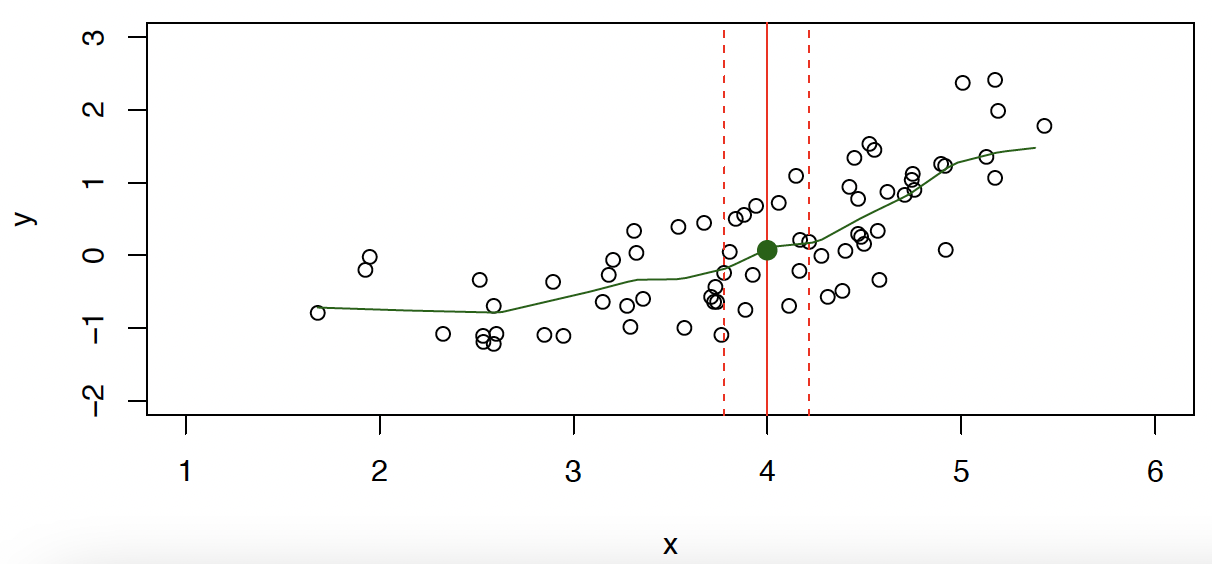
- Nearest neighbor averaging can be pretty good for small .
i.e. and large-ish .
最近邻平均对于较小的 来说是相当不错的
例如, 和 较大的 - Nearest neighbor methods can be lousy when is large.
当 很大时,最近邻方法可能很糟糕。
Reason: the curse of dimensionality. Nearest neighbors tend to be far away in high dimensions.
原因:维度诅咒。在高维空间中,最近的邻居往往离得很远。
# Parametric and Structured Models 参数化和结构化模型
The linear model is an important example of a parametric model:
线性模型是参数模型的一个重要示例:
- A linear model is specified in terms of parameters .
线性模型由 参数 指定。 - We estimate the parameters by fitting the model to training data.
通过拟合训练数据来估计模型的参数。 - Although it is almost never correct, a linear model often serves as a good and interpretable approximation to the unknown true function .
尽管线性模型几乎从来都不是正确的,但它通常是未知真函数 的一个很好的、可解释的近似。
We can also estimate with non-parametric methods.
我们也可以用非参数方法估计。
- do not make explicit assumptions about the functional form of .
不要对 的函数形式做明确的假设。 - Seek an estimate of that gets as close to the data points as possible without being too rough or wiggly.
寻求一个 的估计,尽可能接近数据点,而不是太粗糙或扭曲。
However, we will focus on parametric models.
将关注参数模型。
A linear model gives a reasonable fit here
线性模型... 给出了一个合理的拟合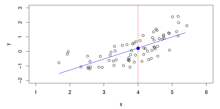
A quadratic model fits slightly better.
二次模型... 更适合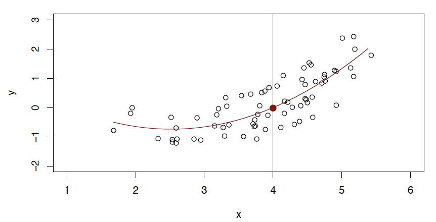
Another Example: Revisit Income example
收入例子:
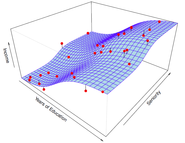
Red points are simulated values for income from the model . is the blue surface.
红点是模型 的收入模拟值, 是蓝色表面。
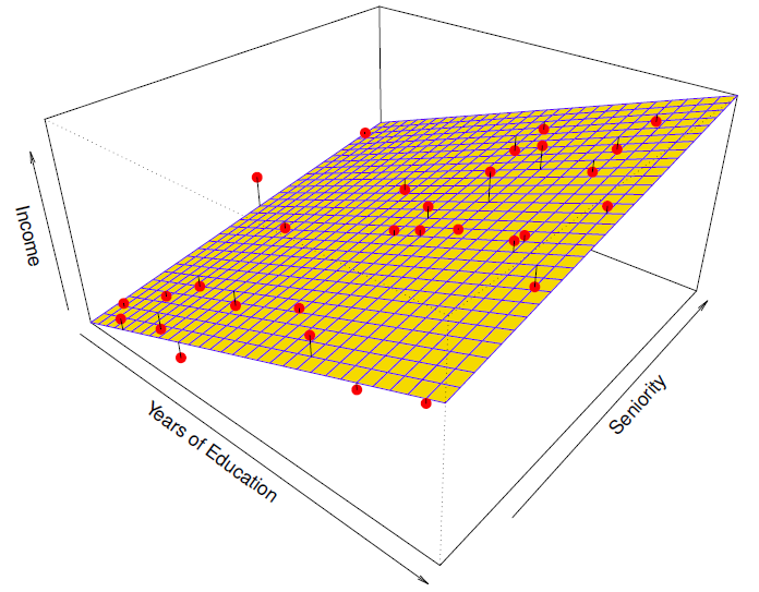
Linear regression model fitt to the simulated data.
线性回归模型符合模拟数据。
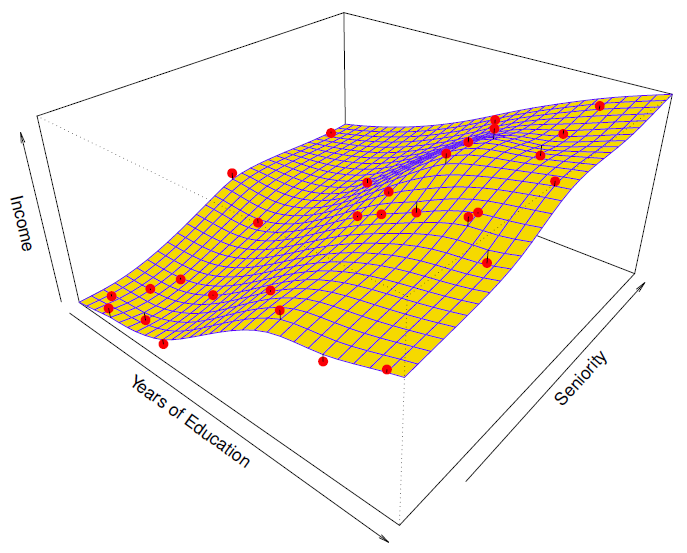
More flexible regression model fit to the simulated data.
更灵活的回归模型... 适合模拟数据。
Here we use a technique called a thin-plate spline to fit a flexible surface.
这里我们使用一种叫做薄板样条的技术来适应一个灵活的表面。
Even more flexible spline regression model fit to the simulated data.
更灵活的样条回归模型... 适合模拟数据。
Here the tted model makes no errors on the training data! Also known as overtting .
在这里,tted 模型在训练数据上没有错误!也被称为 overtting 。
# Prediction Accuracy VS Interpretability 预测精度 VS 可解释性
- Less flexible methods 不太灵活的方法
- more restrictive, relatively small range of shapes for .
限制更多, 形状范围相对较小
E.g. linear regression: easy to understand the relationship between and .
容易理解 和 之间的关系 - More flexible methods 更灵活的方法
- can generate a wider range of possible shapes to estimate .
可以生成更大范围的可能形状来估计
E.g. thin-plate splines: lead to such complicated estimates of that it is difficult to understand how any individual predictor is associated with the response.
薄板样条:导致如此复杂的 估计,以至于很难理解任何单个预测因子如何与响应相关联。
Should we use more flexible models to get better accuracy?
我们应该使用更灵活的模型来获得更好的准确性吗?
Often more accurate prediction using a less flexible method. Why?
通常使用不太灵活的方法进行更准确的预测。为什么?
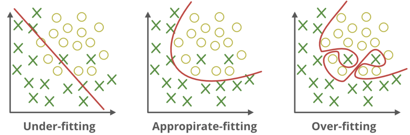
# Good Fit VS. Overfitting or Underfitting 良好拟合 VS 过拟合或欠拟合
# Assessing Model Accuracy 评定模型准确度
There is no free lunch in statistics!
统计学里没有免费的午餐!
No one method dominates all others over all possible data sets.
在所有可能的数据集中,没有一种方法优于所有其他方法。
Important task: decide, for any given set of data, which method produces the best results.
重要任务:决定,对于任何给定的数据集,哪种方法产生最好的结果。Note: Selecting the best approach can be one of the most challenging parts of performing statistical learning in practice.
注意:选择最佳方法可能是统计学习实践中最具挑战性的部分之一。Need: measure how well predictions match observed data.
需求:衡量预测与观测数据的匹配程度。
Quantify the extent to which the predicted response value for a given observation is close to the true response value for that observation.
量化给定观测值的预测响应值,在多大程度上,接近观测值的真实响应值。
# Measuring quality of fit 评价拟合质量
# regression setting 回归设置
Mean Squared Error MSE 均方误差
where is the prediction that gives for the th observation.
其中 是 对第 个观测值的预测。
Suppose we fit a model to some training data
假设我们将一个模型 与一些训练数据相匹配
However, this may be biased toward more overfit models.
然而,这可能偏向于更多的超拟合模型。
What is the accuracy of the predictions that we obtain when we apply our method to previously unseen test data?
当我们将我们的方法应用于以前未见的测试数据时,我们获得的预测的准确性是什么?
# test MSE 测试 MSE
Instead we should, if possible, compute it using fresh.red} test data $Te=\left\{x_{i}, y_{i}\right\}_{1}$ :
相反,如果可能的话,我们应该使用新的测试数据来计算它:
- Scenario: test data available; minimize test MSE on that set.
场景:测试数据可用;最小化该集合上的测试 MSE 。 - Scenario: no test observations available; minimizes training MSE .
场景:没有可用的测试观察;最小化训练 MSE 。

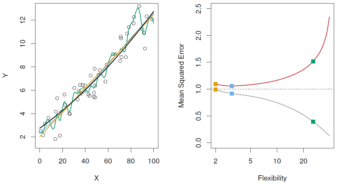
Left: Data simulated from , shown in black.
左图:从 模拟的数据,以黑色显示。
Three estimates of f are shown: the linear regression line (orange curve), and two smoothing spline fits (blue and green curves).
给出了 的三个估计值:线性回归线 (橙色曲线) 和两个平滑样条拟合 (蓝色和绿色曲线)。
Right: Red curve on right is , grey curve is .
右图:红色曲线是,灰色曲线是。
Orange, blue and green curves/squares correspond to fits of different flexibility.
橙色、蓝色和绿色曲线 / 正方形对应于不同灵活性的配合。
Here the truth is smoother, so the smoother fit and linear model do really well.
这里的实际是更平滑的,所以更平滑的拟合和线性模型做得很好。
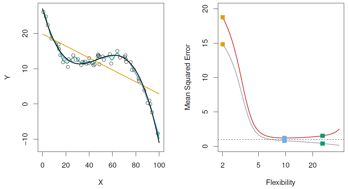
Here the truth is wiggly and the noise is low, so the more flexible fits do the best.
这里的实际是摆动且低噪音,所以更灵活的拟合是最好的。
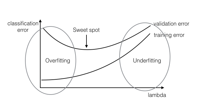
# A Fundamental Conclusion 基本结论
- Increase in model flexibility
增加模型的灵活性- decrease in 减少
- depends on the truth, most case you will see a U-shape
取决于事实,大多数情况下你会看到一个 U 型
- Overfitting: small + large
过拟合 - What to do if no test data available?
没有测试数据怎么办?- Cross-validation: a method for estimating test MSE using training data. (We will learn later)
交叉验证:一种利用训练数据估计测试均方误差的方法。(我们将在后面学习) - Partition the data
分割数据
- Cross-validation: a method for estimating test MSE using training data. (We will learn later)
# Classification Setting 分类设置
Here the response variable is qualitative
这里的响应变量 是定性的
e.g. email is one of (ham=good email), digit class is one of
例如邮件是... 数字类是... 中的一个
Typically we measure the performance of using the misclassication error rate:
通常,我们使用误分类错误率来衡量 的性能:There are several classfiers: the Bayes classifier, support-vector machines Logistic regression, k-nearest neighbour, decision trees, etc.
有几种分类器:贝叶斯分类器、支持向量机 Logistic 回归、k 近邻、决策树等。Some other measures needed. (Why? )
还需要一些其他措施。(为什么?)